Cloud SQL Query Processing
Queries are processed using cells on the Oracle Big Data Service cluster.
About Smart Scan for Big Data Sources
Oracle external tables do not have traditional indexes. Queries against these external tables typically require a full table scan. The Oracle Cloud SQL processing agent on the DataNodes of the Hadoop cluster extends Smart Scan capabilities (such as filter-predicate off-loads) to Oracle external tables. Smart Scan has been used for some time on the Oracle Exadata Database Machine to do column and predicate filtering in the Storage Layer before query results are sent back to the Database Layer. In Cloud SQL, Smart Scan is a final filtering pass done locally on the Hadoop server to ensure that only requested elements are sent to Cloud SQL Query Server. Cloud SQL cells running on the Hadoop DataNodes are capable of doing Smart Scans against various data formats in HDFS, such as CSV text, Avro, and Parquet.
This implementation of Smart Scan leverages the massively parallel processing power of the Hadoop cluster to filter data at its source. It can preemptively discard a huge portion of irrelevant data — up to 99 percent of the total. This has several benefits:
-
Greatly reduces data movement and network traffic between the cluster and the database.
-
Returns much smaller result sets to the Oracle Database server.
-
Aggregates data when possible by leveraging scalability and cluster processing.
Query results are returned significantly faster. This is the direct result of reduced traffic on the network and reduced load on Oracle Database.
About Storage Indexes
For data stored in HDFS, Oracle Cloud SQL maintains Storage Indexes automatically, which is transparent to Oracle Database. Storage Indexes contain the summary of data distribution on a hard disk for the data that is stored in HDFS. Storage Indexes reduce the I/O operations cost and the CPU cost of converting data from flat files to Oracle Database blocks. You can think of a storage index as a negative index. It tells Smart Scan that data does not fall within a block of data, which enables Smart Scan to skip reading that block. This can lead to significant I/O avoidance.
Storage Indexes can be used only for the external tables that are based on HDFS and are created using either the ORACLE_HDFS driver or the ORACLE_HIVE driver. Storage Indexes cannot be used for the external tables that use StorageHandlers, such as Apache HBase and Oracle NoSQL.
A Storage Index is a collection of in-memory region indexes, and each region index stores summaries for up to 32 columns. There is one region index for each split. The content stored in one region index is independent of the other region indexes. This makes them highly scalable, and avoids latch contention.
Storage Indexes maintain the minimum and maximum values of the columns of a region for each region index. The minimum and maximum values are used to eliminate unnecessary I/O, also known as I/O filtering. The cell XT granule I/O bytes saved by the Storage Indexes statistic, available in the V$SYSSTAT view, shows the number of bytes of I/O saved using Storage Indexes.
Queries using the following comparisons are improved by the Storage Indexes:
-
Equality (=)
-
Inequality (<, !=, or >)
-
Less than or equal (<=)
-
Greater than or equal (>=)
-
IS NULL
-
IS NOT NULL
Storage Indexes are built automatically after the Oracle Cloud SQL service receives a query with a comparison predicate that is greater than the maximum or less than the minimum value for the column in a region.
-
The effectiveness of Storage Indexes can be improved by ordering the rows in a table based on the columns that frequently appear in the
WHEREquery clause. -
Storage Indexes work with any nonlinguistic data type, and work with linguistic data types similar to nonlinguistic index.
Elimination of Disk I/O with Storage Indexes
The following figure shows a table and region indexes. The values in column B in the table range from 1 to 8. One region index stores the minimum 1, and the maximum of 5. The other region index stores the minimum of 3, and the maximum of 8.
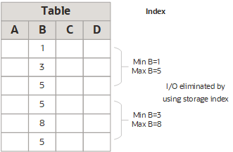
WHERE clause of the query.SELECT *
FROM TABLE
WHERE B < 2;Improved Join Performance Using Storage Indexes
Using Storage Indexes allows table joins to skip unnecessary I/O operations. For example, the following query would perform an I/O operation and apply a Bloom filter to only the first block of the fact table. Bloom filters are the key to improved join performance. In the example, a predicate is on the dimension table, not the fact table. The Bloom filter is created based on dim.name=Hard drive and this filter is then applied to the fact table. Therefore, even though the filter is on the dimension table, you are able to filter the data at its source (Hadoop) based on the results of the dimension query. This also enables optimizations such as Storage Indexes to engage.
SELECT count(*)
FROM fact, dimension dim
WHERE fact.m=dim.m and dim.product="Hard drive";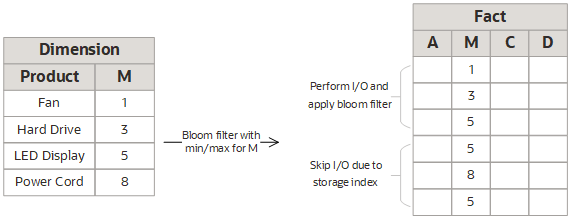
The I/O for the second block of the fact table is completely eliminated by Storage Indexes as its minimum/maximum range (5,8) is not present in the Bloom filter.
About Predicate Pushdown
Many big data systems support some level of predicate off-loading, either through the file type itself (for example, Apache Parquet), or through Hive's partitioning and StorageHandler APIs. Oracle Cloud SQL takes advantage of these off-load capabilities by pushing predicates from Oracle Database into supporting systems. For example, predicate pushdown enables the following automatic behaviors:
-
Queries against partitioned Hive tables are pruned, based on filter predicates on partition columns.
-
Queries against Apache Parquet and Apache ORC files reduce I/O by testing predicates against the internal index-like structures contained within these file formats.
Note
Parquet files must be created using Hive or Spark. Parquet files created using Apache Impala are missing the statistics required for predicate pushdown to engage. -
Queries against Oracle NoSQL Database or Apache HBase use SARGable predicates to drive subscans of data in the remote data store.
Required Datatypes to Enable Predicate Pushdown
Predicate pushdown requires that certain mappings between Hive Datatypes and Oracle Datatypes be present. These mappings are described in the following table.
| Hive Datatype | Mapped to Oracle Datatype |
|---|---|
|
CHAR(m) |
CHAR(n), VARCHAR2(n) where n is >= m |
|
VARCHAR(m) |
CHAR(n), VARCHAR2(n) where n is >= m. |
|
string |
CHAR(n), VARCHAR2(n) |
|
DATE |
DATE |
|
TIMESTAMP |
TIMESTAMP(9) Hive TIMESTAMP has nanoseconds, 9 digit fractional seconds. |
|
TINYINT |
NUMBER(3) preferably, but NUMBER or NUMBER(n) for any value of n is valid. |
|
SMALLINT |
NUMBER(5) preferably, but NUMBER or NUMBER(n) for any value of n is valid. |
|
INT |
NUMBER(10) preferably, but NUMBER or NUMBER(n) for any value of n is valid. |
|
BIGINT |
NUMBER(19) preferably, but NUMBER or NUMBER(n) for any value of n is OK. |
|
DECIMAL(m) |
NUMBER(n) where m = n preferably, but NUMBER or NUMBER(n) for any value of n is valid. |
|
FLOAT |
BINARY_FLOAT |
|
DOUBLE |
BINARY_DOUBLE |
|
BINARY |
RAW(n) |
|
BOOLEAN |
CHAR(n), VARCHAR2(n) where n is >= 5, values 'TRUE', 'FALSE' |
|
BOOLEAN |
NUMBER(1) preferably, but NUMBER or NUMBER(n) for any value of n is valid. Values 0 (false), 1 (true). |
About Pushdown of Character Large Object (CLOB) Processing
Queries against Hadoop data may involve processing large objects with potentially millions of records. It is inefficient to return these objects to Oracle Database for filtering and parsing. Oracle Cloud SQL can provide significant performance gains by pushing CLOB processing down to its own processing cells on the Hadoop cluster. Filtering in Hadoop reduces the number of rows returned to Oracle Database. Parsing reduces the amount of data returned from a column within each filtered row.
You can disable or reenable CLOB processing pushdown to suit your own needs.
This functionality currently applies only to JSON expressions returning CLOB data. The eligible JSON filter expressions for storage layer evaluation include simplified syntax, JSON_VALUE, and JSON_QUERY.
The same support will be provided for other CLOB types (such as substr and instr) as well as for BLOB data in a future release.
Cloud SQL can push processing down to Hadoop for CLOBs within these size constraints:
-
Filtering for CLOB columns up to 1 MB in size.
The actual amount of data that can be consumed for evaluation in the storage server may vary, depending on the character set used.
-
Parsing for columns up to 32 KB.
This limit refers to the select list projection from storage for the CLOB datatype.
Processing falls back to Oracle Database only when column sizes exceed these two values.
JSON Document Processing
{"ponumber":9764,"reference":"LSMITH-20141017","requestor":"Lindsey Smith","email": "Lindsey@myco.com", "company":"myco" …}CREATE TABLE POS_DATA
( pos_info CLOB )
ORGANIZATION EXTERNAL
( TYPE ORACLE_HDFS
DEFAULT DIRECTORY DEFAULT_DIR
LOCATION ('/data/pos/*')
)
REJECT LIMIT UNLIMITED;SELECT p.pos_info.email, p.pos_info.requestor
FROM POS_DATA p
WHERE p.pos_info.company='myco'
The query example above engages two data elimination optimizations:
-
The data is filtered by Cloud SQL cells in the Hadoop cluster. Only records pertaining to the company
mycoare parsed (and after parsing only selected data from these records is returned to the database). -
Cloud SQL cells in the cluster parse the filtered set of records and from each record only the values for the two attributes requested (
p.pos_info.emailandp.pos_info.requestor) are returned to the database.
The table below shows some other examples where CLOB processing pushdown is supported. Remember that projections (references on the select side of the CLOB column) are limited to 32 KB of CLOB data, while predicate pushdown is limited to 1 MB of CLOB data.
| Query | Comment |
|---|---|
SELECT count(*) FROM pos_data p WHERE pos_info is json; |
In this case, the predicate ensures that only columns that comply with JSON format are returned. |
SELECT pos_info FROM pos_data p WHERE pos_info is json; |
The same predicate as in the previous case, but now the CLOB value is projected. |
SELECT json_value(pos_info, '$.reference') FROM pos_data p WHERE json_value(pos_info, '$.ponumber') > 9000 |
Here, the predicate is issued on a field of the JSON document, and we also execute a JSON value to retrieve field "reference" on top of the projected CLOB JSON value. |
SELECT p.pos_info.reference FROM pos_data p WHERE p.pos_info.ponumber > 9000; |
This is functionally the same query as the previous example, but expressed in simplified syntax. |
SELECT p.pos_info.email FROM po_data p WHERE json_exists(pos_info, '$.requestor') and json_query(pos_info, '$.requestor') is not null; |
This example shows how json_exists and json_query can also be used as predicates. |
About Aggregation Offload
Oracle Cloud SQL uses Oracle In-Memory technology to push aggregation processing down to the Cloud SQL cells. This enables Cloud SQL to leverage the processing power of the Hadoop cluster for distributing aggregations across the cluster nodes.
The performance gains can be significantly faster compared to aggregations that do not offload, especially when there are a moderate number of summary groupings. For single table queries, the aggregation operation should consistently offload.
Cloud SQL cells support single-table and multi-table aggregations (for example, dimension tables joining to a fact table). For multi-table aggregations, Oracle Database uses the key vector transform optimization in which the key vectors are pushed to the cells for the aggregation process. This transformation type is useful for star join SQL queries that use typical aggregation operators (such as SUM, MIN, MAX, and COUNT), which are common in business queries.
A vector transformation query is a more efficient query that uses a Bloom filter for joins. When you use a vector transformed query with Cloud SQL cells, the performance of joins in the query is enhanced by the ability to offload filtration for rows used for aggregation. You see a KEY VECTOR USE operation in the query plan during this optimization.
In Cloud SQL cells, vector transformed queries benefit from more efficient processing due to the application of group-by columns (key vectors) to the Cloud SQL Storage Index.
-
Missing predicate
If theSYS_OP_VECTOR_GROUP_BYpredicate is missing in the explain plan, aggregation offload is affected. The predicate can be missing due to the following reasons:-
Presence of a disallowed intervening row source between the table scan and group-by row sources.
-
The table scan does not produce rowsets.
-
Presence of an expression or data type in the query that can not be offloaded.
-
Vector group-by is manually disabled.
-
The table of table scan or configuration does not expect gains from aggregation offload.
-
-
Missing smart scan
The cell interconnect bytes returned by XT smart scan and cell XT granules requested for predicate offload statistics must be available.
-
Missing key vectors
The limit on the data transmitted to the cells is 1 MB. If this threshold is exceeded, then queries can benefit from intelligent key vector filtering but not necessarily offloaded aggregation. This condition is known as Key Vector Lite mode. Due to their large size, some of the key vectors are not fully offloaded. They get offloaded in lite mode along with the key vectors that do not support aggregation offload. Key vectors are not completely serialized in lite mode. The vector group-by offload is disabled when key vectors are offloaded in lite mode.
See Optimizing Aggregation in Oracle Database In-Memory Guide for information about how aggregation works in Oracle Database.
About Cloud SQL Statistics
Oracle Cloud SQL provides a number of statistics that can contribute data for performance analyses.
Five Key Cell XT and Storage Index Statistics
If a query is off-loadable, the following XT-related statistics can help you determine what kind of I/O savings you can expect from the offload and from Smart Scan.
-
cell XT granules requested for predicate offload
The number of granules requested depends on a number of factors, including the HDFS block size, Hadoop data source splittability, and the effectiveness of Hive partition elimination.
-
cell XT granule bytes requested for predicate offload
The number of bytes requested for the scan. This is the size of the data on Hadoop to be investigated after Hive partition elimination and before Storage Index evaluation.
-
cell interconnect bytes returned by XT smart scan
The number of bytes of I/O returned by an XT smart scan to Oracle Database.
-
cell XT granule predicate offload retries
The number of times that a Cloud SQL process running on a DataNode could not complete the requested action. Cloud SQL automatically retries failed requests on other DataNodes that have a replica of the data. The retries value should be zero.
-
cell XT granule IO bytes saved by storage index
The number of bytes filtered out by storage indexes at the storage cell level. This is data that was not scanned, based on information provided by the storage indexes.
You can check these statistics before and after running queries as follows. This example shows the values at null, before running any queries.
SQL> SELECT sn.name,ms.value
FROM V$MYSTAT ms, V$STATNAME sn
WHERE ms.STATISTIC#=sn.STATISTIC# AND sn.name LIKE '%XT%';

NAME                                                      VALUE
-----------------------------------------------------     -----
cell XT granules requested for predicate offload          0
cell XT granule bytes requested for predicate offload     0
cell interconnect bytes returned by XT smart scan         0
cell XT granule predicate offload retries                 0
cell XT granule IO bytes saved by storage index           0
You can check some or all of these statistics after execution of a query to test the effectiveness of the query, as in:
SQL> SELECT n.name, round(s.value/1024/1024)
FROM v$mystat s, v$statname n
WHERE s.statistic# IN (462,463)
AND s.statistic# = n.statistic#;

cell XT granule bytes requested for predicate offload  32768
cell interconnect bytes returned by XT smart scan   32
Five Aggregation Offload Statistics
The following statistics can help you analyze the performance of aggregation offload.
-
vector group by operations sent to cell
The number of times aggregations can be offloaded to the cell.
-
vector group by operations not sent to cell due to cardinality
The number of scans that were not offloaded because of large wireframe.
-
vector group by rows processed on cell
The number of rows that were aggregated on the cell.
-
vector group by rows returned by cell
The number of aggregated rows that were returned by the cell.
-
vector group by rowsets processed on cell
The number of rowsets that were aggregated on the cell.
You can review these statistics by running the queries as follows:
SQL> SELECT count(*) FROM bdsql_parq.web_sales;

  COUNT(*)
----------
 287301291

SQL> SELECT substr(n.name, 0,60) name, u.value
FROM v$statname n, v$mystat u
WHERE ((n.name LIKE 'key vector%') OR
       (n.name LIKE 'vector group by%') OR
       (n.name LIKE 'vector encoded%') OR
       (n.name LIKE '%XT%') OR
       (n.name LIKE 'IM %' AND n.name NOT LIKE '%spare%'))
      AND u.sid=userenv('SID')
      AND n.STATISTIC# = u.STATISTIC#
      AND u.value > 0;


NAME                                                      VALUE
-----------------------------------------------------     -----
cell XT granules requested for predicate offload          808
cell XT granule bytes requested for predicate offload     2.5833E+10
cell interconnect bytes returned by XT smart scan         6903552
vector group by operations sent to cell                   1
vector group by rows processed on cell                    287301291
vector group by rows returned by cell                     808
Nine Key Vector Statistics
The following statistics can help you analyze the effectiveness of key vectors that were sent to the cell.
-
key vectors sent to cell
The number of key vectors that were offloaded to the cell.
-
key vector filtered on cell
The number of rows that were filtered out by a key vector on the cell.
-
key vector probed on cell
The number of rows that were tested by a key vector on the cell.
-
key vector rows processed by value
The number of join keys that were processed by using their value.
-
key vector rows processed by code
The number of join keys that were processed by using the dictionary code.
-
key vector rows filtered
The number of join keys that were skipped due to skip bits.
-
key vector serializations in lite mode for cell
The number of times a key vector was not encoded due to format or size.
-
key vectors sent to cell in lite mode due to quota
The number of key vectors that were offloaded to the cell for non-exact filtering due to the 1 MB metadata quota.
-
key vector efilters created
A key vector was not sent to a cell, but an efilter (similar to a Bloom filter) was sent.
You can review these statistics by running the queries as follows:
SELECT substr(n.name, 0,60) name, u.value
FROM v$statname n, v$mystat u
WHERE ((n.name LIKE 'key vector%') OR
       (n.name LIKE 'vector group by%') OR
       (n.name LIKE 'vector encoded%') OR
       (n.name LIKE '%XT%'))
      AND u.sid=userenv('SID')
      AND n.STATISTIC# = u.STATISTIC#


NAME                                                      VALUE
-----------------------------------------------------     -----
cell XT granules requested for predicate offload          250
cell XT granule bytes requested for predicate offload     61,112,831,993
cell interconnect bytes returned by XT smart scan         193,282,128
key vector rows processed by value                        14,156,958
key vector rows filtered                                  9,620,606
key vector filtered on cell                               273,144,333
key vector probed on cell                                 287,301,291
key vectors sent to cell                                  1
key vectors sent to cell in lite mode due to quota        1
key vector serializations in lite mode for cell           1
key vector efilters created                               1
The Big Data SQL Quick Start blog, published in The Data Warehouse Insider , shows how to use these statistics to analyze the performance of Big Data SQL. Cloud SQL and Big Data SQL share the same underlying technology, so the same optimization rules apply. See Part 2, Part 7, and Part 10.