Data Flow Integration with Data Science

With Data Flow, you can configure Data Science notebooks to run applications interactively against Data Flow.

Data Flow uses fully managed Jupyter Notebooks to enable data scientists and data engineers to create, visualize, collaborate, and debug data engineering and data science applications. You can write these applications in Python, Scala, and PySpark. You can also connect a Data Science notebook session to Data Flow to run applications. The Data Flow kernels and applications run on Oracle Cloud Infrastructure Data Flow.

Apache Spark is a distributed compute system designed to process data at scale. It supports large-scale SQL, batch, and stream processing, and machine learning tasks. Spark SQL provides database-like support. To query structured data, use Spark SQL. It's an ANSI standard SQL implementation.

Data Flow Sessions support autoscaling Data Flow cluster capabilities. For more information, see Autoscaling in the Data Flow documentation.

Data Flow Sessions support the use of conda environments as customizable Spark runtime environments.
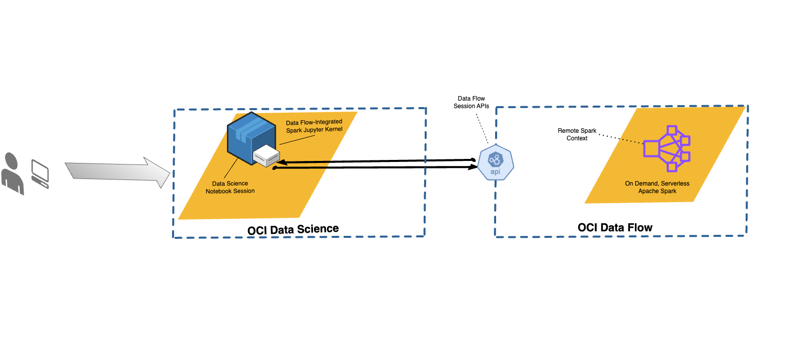
Figure 1. Data Science Notebook to Data Flow
A Data Science notebook uses Data Flow Magic to send requets to Data Flow using the NotebookSession APIs to run Spark code on a Data Flow server.
Limitations
  • Data Flow Sessions last up to 7 days or 10,080 mins (maxDurationInMinutes).

  • Data Flow Sessions have a default idle timeout value of 480 mins (8 hours) (idleTimeoutInMinutes). You can configure a different value.
  • The Data Flow Session is only available through a Data Science Notebook Session.
  • Only Spark version 3.5.0 and 3.2.1 are supported.
Tip

Watch the tutorial video on using Data Science with Data Flow Studio. Also see the Oracle Accelerated Data Science SDK documentation for more information on integrating Data Science and Data Flow.

Installing the Conda Environment

Follow theses steps to use Data Flow with Data Flow Magic.

  1. Create or open a notebook session in Data Science.
    • The notebook session must be in the region where the service was enabled for the tenancy.
    • The notebook session must be in the compartment of the dynamic group of notebook sessions.
  2. Install and activate the pyspark32_p38_cpu_v3 conda environment in the notebook session:
    copy odsc conda install -s pyspark32_p38_cpu_v3
    Note

    We recommend installing the updated conda environment pyspark32_p38_cpu_v3, as it includes support for automatically restarting sessions that have stopped because they have exceeded the maximum timeout duration.

    The previous stable conda environment was pyspark32_p38_cpu_v2.

  3. Activate the pyspark32_p38_cpu_v3 conda environment:
    source activate /home/datascience/conda/pyspark32_p38_cpu_v3

Using Data Flow with Data Science

Follow these steps to run an application using Data Flow with Data Science.

  • Ensure you have the policies set up to use a notebook with Data Flow.

  • Ensure you have the Data Science policies set up correctly.

  • For a list of all the supported commands, use the %help command.
  • The commands in the following steps apply for both Spark 3.5.0 and Spark 3.2.1. Spark 3.5.0 is used in the examples. Set the value of sparkVersion according to the version of Spark used.
  1. Set up authentication in ADS.
    • The ADS SDK is used to control the authentication type used in in Data Flow Magic.
    • The API KEY authentication is used by default. To change authentication type, use the ads.set_auth("resource_principal") command:
      import ads
      ads.set_auth("resource_principal") # Supported values: resource_principal, api_key
  2. Load the Data Flow Magic extension
    %load_ext dataflow.magics
  3. (Optional) Create a Data Flow session using the magic command, %create_session:
    Common Session
    This example shows how to create a new session on flexible shapes:
    import json
    command = {
        "compartmentId": "<compartment_ocid>",
        "displayName": "<session_name>",
        "language": "PYTHON",
        "sparkVersion": "3.5.0",
        "driverShape": "VM.Standard.E3.Flex",
        "executorShape": "VM.Standard.E3.Flex",
        "driverShapeConfig":{"ocpus":1,"memoryInGBs":16},
        "executorShapeConfig":{"ocpus":1,"memoryInGBs":16},
        "numExecutors": 1,
        "type": "SESSION",
        "logsBucketUri": "oci://<bucket>@<namespace>/",
    }
    command = f'\'{json.dumps(command)}\''
     
    %create_session -l python -c $command
    Session with archive URI
    import json
    command = {
        "compartmentId": "<compartment_ocid>",
        "displayName": "<session_name>",
        "language": "PYTHON",
        "sparkVersion": "3.5.0",
        "driverShape": "VM.Standard.E3.Flex",
        "executorShape": "VM.Standard.E3.Flex",
        "driverShapeConfig":{"ocpus":1,"memoryInGBs":16},
        "executorShapeConfig":{"ocpus":1,"memoryInGBs":16},
        "numExecutors": 1,
        "type": "SESSION",
        "logsBucketUri": "oci://<bucket>@<namespace>",
        "archiveUri": <oci://<bucket>@<namespace>/archive.zip"
    }
    command = f'\'{json.dumps(command)}\''
     
    %create_session -l python -c $command
    Session with a custom conda environment
    import json
    command = {
        "compartmentId": "<compartment_ocid>",
        "displayName": "<session_name>",
        "language": "PYTHON",
        "sparkVersion": "3.5.0",
        "driverShape": "VM.Standard.E3.Flex",
        "executorShape": "VM.Standard.E3.Flex",
        "driverShapeConfig":{"ocpus":1,"memoryInGBs":16},
        "executorShapeConfig":{"ocpus":1,"memoryInGBs":16},
        "numExecutors": 1,
        "type": "SESSION",
        "logsBucketUri": "oci://<bucket>@<namespace>",
        "configuration": {
            "spark.archives": "oci://<bucket>@<namespace>/conda_pack/<pack_name>"
        },
    }
    command = f'\'{json.dumps(command)}\''
     
    %create_session -l python -c $command
    Session with Metastore
    import json
    command = {
        "compartmentId": "<compartment_ocid>",
        "displayName": "<session_name>",
        "language": "PYTHON",
        "sparkVersion": "3.5.0",
        "driverShape": "VM.Standard.E3.Flex",
        "executorShape": "VM.Standard.E3.Flex",
        "driverShapeConfig":{"ocpus":1,"memoryInGBs":16},
        "executorShapeConfig":{"ocpus":1,"memoryInGBs":16},
        "numExecutors": 1,
        "type": "SESSION",
        "logsBucketUri": oci://<bucket>@<namespace>",
        "metastoreId": "<ocid1.datacatalogmetastore.oc1.iad...>",
        "configuration": {
            "spark.archives": "oci://<bucket>@<namespace>/conda_pack/<pack_name>"
        },
    }
    command = f'\'{json.dumps(command)}\''
     
    %create_session -l python -c $command
  4. (Optional) Use an existing Data Flow session:
    Use the %use_session command. Copy the OCID from the Console.
    %use_session -s <session_OCID> -r <region_name>
  5. Configure the session using the %config_session command:
    • To see the current configuration:
      %config
    • To change the drivers and executors:
      %configure_session -i '{"driverShape": "VM.Standard2.1", "executorShape": "VM.Standard2.1", "numExecutors": 1}'
    • To apply Autoscaling:
      %configure_session -i '{"driverShape": "VM.Standard2.1",\
      "executorShape": "VM.Standard2.1", "numExecutors": 16,\
      "sparkVersion":"3.5.0",\
      "configuration":{"spark.dynamicAllocation.enabled":"true",\
      "spark.dynamicAllocation.shuffleTracking.enabled":"true",\
      "spark.dynamicAllocation.minExecutors":"16",\
      "spark.dynamicAllocation.maxExecutors":"54",\
      "spark.dynamicAllocation.executorIdleTimeout":"60",\
      "spark.dynamicAllocation.schedulerBacklogTimeout":"60",\
      "spark.dataflow.dynamicAllocation.quotaPolicy":"max"} \
      }'
      You can also apply an autoscaling policy when you create a session.
  6. (Optional) To activate an existing session, use the %activate_session command:
    %activate_session -l python -c 
    '{"compartmentId": "<Compartment_OCID>",
        "displayName": "<Name>",
        "applicationId": "<Application_OCID>"
    }'
  7. To stop a session, use the %stop_session command:
    %stop_session

Customizing a Data Flow Spark Environment with a Conda Environment

You can use a published conda environment as a runtime environment.

  1. Install Spark 3.5.0 and Data Flow in the notebook session:
    odsc conda install -s pyspark32_p38_cpu_v3
  2. Install the libraries using conda.
  3. Publish the conda environment:
    odsc conda publish -s pyspark32_p38_cpu_v3
  4. Start the Data Flow cluster, for example:
    %create_session -l python -c '{"compartmentId":"<your-compartment-ocid>", \
    "displayName":"<your-display-name>",\
    "sparkVersion":"3.5.0", \
    "language":"PYTHON", \
    "type": "SESSION",\
    "driverShape":"VM.Standard2.1", \
    "executorShape":"VM.Standard2.1",\
    "numExecutors":1,\
    "configuration": {"spark.archives":"oci://<your-bucket>@<your-tenancy-namespace>/<your-path-to-the-conda-environment>#conda"}}'
    Note

    The session configuration must include the following parameters:
    • "sparkVersion":"3.5.0"
    • "language":"PYTHON"
    • "configuration" with a spark.archives path to the conda environment on object storage.

Running spark-nlp on Data Flow

Follow these steps to install Spark-nlp and run on Data Flow.

You must have completed steps 1 and 2 in Customizing a Data Flow Spark Environment with a Conda Environment. The spark-nlp library is pre-installed in the pyspark32_p38_cpu_v2 conda environment.

  1. Install the pre-trained spark-nlp models and pipelines.

    If you need any pre-trained spark-nlp models, download them and unzip them in the conda environment folder. Data Flow doesn't yet support egress to the public internet. You can't dynamically download pre-trained models from AWS S3 in Data Flow.

    You can download pre-trained models from the model hub as zip archives Unzip the model in the conda environment folder. The example model is https://nlp.johnsnowlabs.com/2021/03/23/explain_document_dl_en.html:
    mkdir /home/datascience/conda/pyspark32_p38_cpu_v2/sparknlp-models
    unzip explain_document_dl_en_3.0.0_3.0_1616473268265.zip -d /home/datascience/conda/pyspark32_p38_cpu_v2/sparknlp-models/
  2. Publish the conda environment, see step 3 in Customizing a Data Flow Spark Environment with a Conda Environment.
  3. Start the Data Flow cluster.

    In a notebook cell running in the notebook session pyspark30_p37_cpu_v5 kernel, double-check the

    spark.jars.packages parameter. It reflects the version of spark-nlp that you have installed.
    %create_session -l python -c '{"compartmentId":" <your-compartment-ocid>", \
    "displayName":"sparknlp",\
    "sparkVersion":"3.2.1", \
    "language":"PYTHON", \
    "type": "SESSION",\
    "driverShape":"VM.Standard2.1", \
    "executorShape":"VM.Standard2.1",\
    "numExecutors":1,\
    "configuration": {"spark.archives":"oci://<your-bucket>@<your-tenancy-namespace>/<your-path-to-the-conda-environment>#conda",\
    "spark.jars.ivy":"/opt/spark/work-dir/conda/.ivy2",\
    "spark.jars.packages": "com.johnsnowlabs.nlp:spark-nlp_2.12:4.1.0"}\
    }'
  4. Test it with a snippet of code from the spark-nlp GitHub repository:
    %%spark
     
    from sparknlp.base import *
    from sparknlp.annotator import *
    from sparknlp.pretrained import PretrainedPipeline
    import sparknlp
     
    # Start SparkSession with Spark NLP
    # start() functions has 3 parameters: gpu, m1, and memory
    # sparknlp.start(gpu=True) will start the session with GPU support
    # sparknlp.start(m1=True) will start the session with macOS M1 support
    # sparknlp.start(memory="16G") to change the default driver memory in SparkSession
    spark = sparknlp.start()
     
    # Download a pre-trained pipeline
    pipeline = PretrainedPipeline('explain_document_dl', lang='en', disk_location="/opt/spark/work-dir/conda/sparknlp-models/")
     
     
    # Your testing dataset
    text = """
    Lawrence Joseph Ellison (born August 17, 1944) is an American business magnate and investor who is the co-founder,
    executive chairman, chief technology officer (CTO) and former chief executive officer (CEO) of the
    American computer technology company Oracle Corporation.[2] As of September 2022, he was listed by
    Bloomberg Billionaires Index as the ninth-wealthiest person in the world, with an estimated
    fortune of $93 billion.[3] Ellison is also known for his 98% ownership stake in Lanai,
    the sixth-largest island in the Hawaiian Archipelago.[4]
    """
     
    # Annotate your testing dataset
    result = pipeline.annotate(text)
     
    # What's in the pipeline
    print(list(result.keys()))
     
    # Check the results
    print(result['entities'])
    The following output is in the notebook cell:
    ['entities', 'stem', 'checked', 'lemma', 'document', 'pos', 'token', 'ner', 'embeddings', 'sentence']
    ['Lawrence Joseph Ellison', 'American', 'American', 'Oracle Corporation', 'Bloomberg Billionaires Index', 'Ellison', 'Lanai', 'Hawaiian Archipelago']

Examples

Here are some examples of using Data FlowMagic.

PySpark

The variable sc represents the Spark and it's available when the %%spark magic command is used. The following cell is a toy example of how to use sc in a Data FlowMagic cell. The cell calls the .parallelize() method which creates an RDD, numbers, from a list of numbers. Information about the RDD is printed. The .toDebugString() method returns a description of the RDD.
%%spark
print(sc.version)
 
numbers = sc.parallelize([4, 3, 2, 1])
print(f"First element of numbers is {numbers.first()}")
print(f"The RDD, numbers, has the following description\n{numbers.toDebugString()}")

Spark SQL

Using the -c sql option lets you run Spark SQL commands in a cell. In this section, the citi bike dataset is used. The following cell reads the dataset into a Spark dataframe and saves it as a table. This example is used to show Spark SQL.

The Citibike dataset is uploaded to object storage. You might need to do the same in your realm.
%%spark
df_bike_trips = spark.read.csv("oci://dmcherka-dev@ociodscdev/201306-citibike-tripdata.csv", header=False, inferSchema=True)
df_bike_trips.show()
df_bike_trips.createOrReplaceTempView("bike_trips")

The following example uses the -c sql option to tell Data FlowMagic that the contents of the cell is SparkSQL. The -o <variable> option takes the results of the Spark SQL operation and stores it in the defined variable. In this case, the

df_bike_trips are a Pandas dataframe that's available to be used in the notebook.
%%spark -c sql -o df_bike_trips
SELECT _c0 AS Duration, _c4 AS Start_Station, _c8 AS End_Station, _c11 AS Bike_ID FROM bike_trips;
Print the first few rows of data:
df_bike_trips.head()
Similarly you can use sqlContext to query the table:
%%spark
df_bike_trips_2 = sqlContext.sql("SELECT * FROM bike_trips")
df_bike_trips_2.show()
Finally, you can describe the table:
%%spark -c sql
SHOW TABLES

Auto-visualization Widget

Data FlowMagic comes with autovizwidget which enables the visualization of Pandas dataframes. The display_dataframe() function takes a Pandas dataframe as a parameter and generates an interactive GUI in the notebook. It has tabs that show the visualization of the data in various forms, such as tabular, pie charts, scatter plots, and area and bar graphs.

The following cell calls display_dataframe() with the df_people dataframe that was created in the Spark SQL section of the notebook:
from autovizwidget.widget.utils import display_dataframe
display_dataframe(df_bike_trips)

Matplotlib

A common task that data scientists perform is to visualize their data. With large datasets, it's usually not possible and is almost always not preferable to pull the data from the Data Flow Spark cluster into the notebook session. This example proves how to use server-side resources to generate a plot and include it in the notebook.

The df_bike_trips dataframe is defined in the session and is reused. To produce a Matplotlib, include the required libraries and generate the plot. Use the %matplot plt magic command to display the plot in the notebook, even though it's rendered on the server-side:
%%spark
import matplotlib.pyplot as plt
df_bike_trips.groupby("_c4").count().toPandas().plot.bar(x="_c4", y="count")
%matplot plt

Further Examples

More examples are available from GitHub with Data Flow samples and Data Science samples.