Data Flow Integration with Data Science
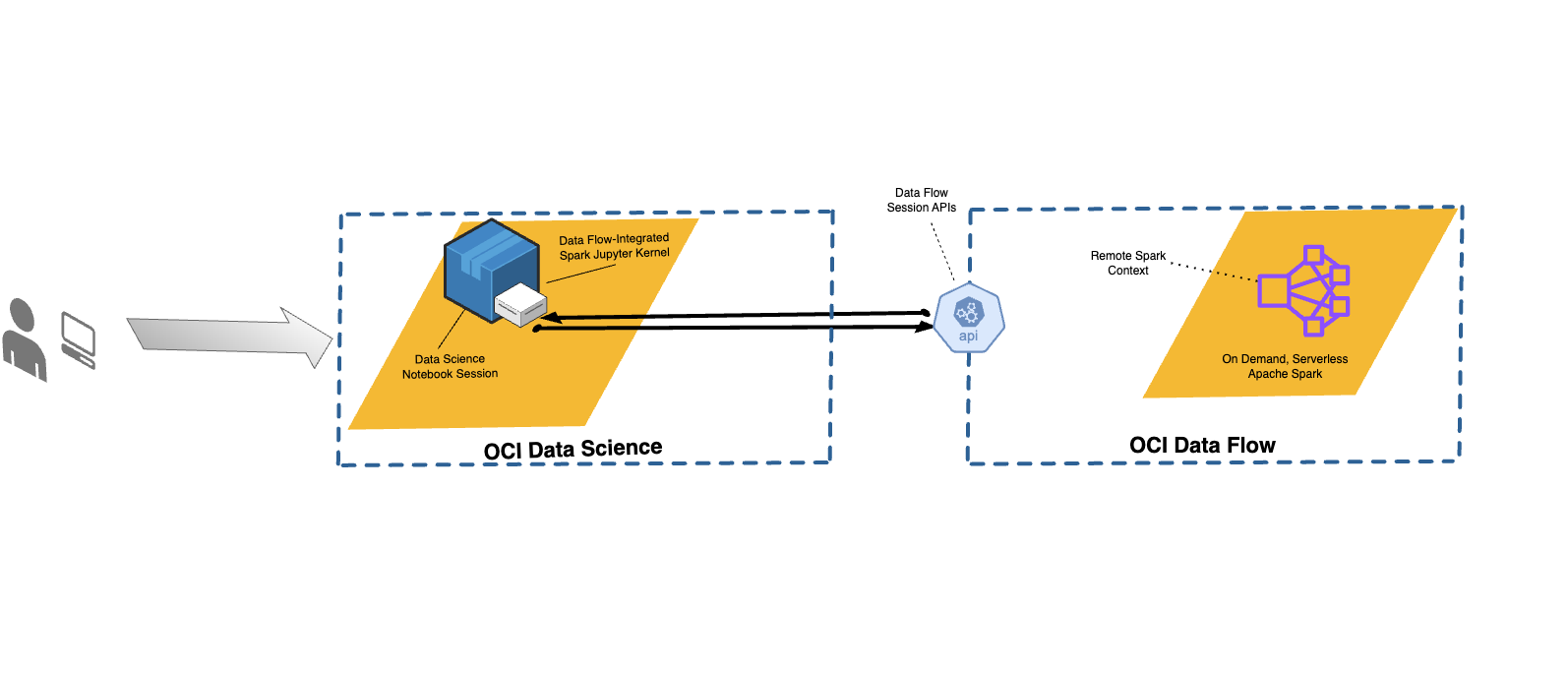
With Data Flow, you can configure Data Science notebooks to run applications interactively against Data Flow.
Data Flow uses fully managed Jupyter Notebooks to enable data scientists and data engineers to create, visualize, collaborate, and debug data engineering and data science applications. You can write these applications in Python, Scala, and PySpark. You can also connect a Data Science notebook session to Data Flow to run applications. The Data Flow kernels and applications run on Oracle Cloud Infrastructure Data Flow .
Apache Spark is a distributed compute system designed to process data at scale. It supports large-scale SQL, batch, and stream processing, and machine learning tasks. Spark SQL provides database-like support. To query structured data, use Spark SQL. It's an ANSI standard SQL implementation.
Data Flow Sessions support autoscaling Data Flow cluster capabilities. For more information, see Autoscaling in the Data Flow documentation.
Data Flow Sessions support the use of conda environments as customizable Spark runtime environments.
- Limitations
-
-
Data Flow Sessions last up to 7 days or 10,080 mins (maxDurationInMinutes).
- Data Flow Sessions have a default idle timeout value of 480 mins (8 hours) (idleTimeoutInMinutes). You can configure a different value.
- The Data Flow Session is only available through a Data Science Notebook Session.
- Only Spark version 3.5.0 and 3.2.1 are supported.
-
Watch the tutorial video on using Data Science with Data Flow Studio. Also see the Oracle Accelerated Data Science SDK documentation for more information on integrating Data Science and Data Flow.
Installing the Conda Environment
Follow theses steps to use Data Flow with Data Flow Magic.
Using Data Flow with Data Science
Follow these steps to run an application using Data Flow with Data Science.
-
Ensure you have the policies set up to use a notebook with Data Flow.
-
Ensure you have the Data Science policies set up correctly.
- For a list of all the supported commands, use the
%helpcommand. - The commands in the following steps apply for both Spark 3.5.0 and Spark 3.2.1.
Spark 3.5.0 is used in the examples. Set the value of
sparkVersionaccording to the version of Spark used.
Customizing a Data Flow Spark Environment with a Conda Environment
You can use a published conda environment as a runtime environment.
Running spark-nlp on Data Flow
Follow these steps to install Spark-nlp and run on Data Flow.
You must have completed steps 1 and 2 in Customizing a Data Flow Spark Environment with a Conda Environment. The spark-nlp library is
pre-installed in the pyspark32_p38_cpu_v2 conda environment.
Examples
Here are some examples of using Data FlowMagic.
PySpark
sc represents the Spark and it's available when the
%%spark magic command is used. The following cell is a toy
example of how to use sc in a Data FlowMagic cell. The cell calls the
.parallelize()
method
which creates an RDD, numbers, from a list
of numbers. Information about the RDD is printed. The
.toDebugString()
method
returns a description of the
RDD.%%spark
print(sc.version)
numbers = sc.parallelize([4, 3, 2, 1])
print(f"First element of numbers is {numbers.first()}")
print(f"The RDD, numbers, has the following description\n{numbers.toDebugString()}")Spark SQL
Using the -c
sql option lets you run Spark SQL commands in a cell. In this section,
the citi bike dataset is used. The following cell reads the
dataset into a Spark dataframe and saves it as a table. This example is used to show
Spark SQL.
%%spark
df_bike_trips = spark.read.csv("oci://dmcherka-dev@ociodscdev/201306-citibike-tripdata.csv", header=False, inferSchema=True)
df_bike_trips.show()
df_bike_trips.createOrReplaceTempView("bike_trips")
The following
example uses the -c sql option to tell Data FlowMagic that the contents of the cell is
SparkSQL. The -o <variable> option takes the results of the
Spark SQL operation and stores it in the defined variable. In this case, the
df_bike_trips are a Pandas dataframe that's available to be
used in the
notebook.%%spark -c sql -o df_bike_trips
SELECT _c0 AS Duration, _c4 AS Start_Station, _c8 AS End_Station, _c11 AS Bike_ID FROM bike_trips;df_bike_trips.head()sqlContext to query the
table:%%spark
df_bike_trips_2 = sqlContext.sql("SELECT * FROM bike_trips")
df_bike_trips_2.show()%%spark -c sql
SHOW TABLESAuto-visualization Widget
Data FlowMagic comes with autovizwidget which enables the
visualization of Pandas dataframes. The display_dataframe()
function takes a Pandas dataframe as a parameter and generates an interactive GUI in
the notebook. It has tabs that show the visualization of the data in various forms,
such as tabular, pie charts, scatter plots, and area and bar graphs.
display_dataframe() with the
df_people dataframe that was created in the Spark SQL section of the
notebook:from autovizwidget.widget.utils import display_dataframe
display_dataframe(df_bike_trips)Matplotlib
A common task that data scientists perform is to visualize their data. With large datasets, it's usually not possible and is almost always not preferable to pull the data from the Data Flow Spark cluster into the notebook session. This example proves how to use server-side resources to generate a plot and include it in the notebook.
%matplot plt magic command to display the plot in the notebook,
even though it's rendered on the
server-side:%%spark
import matplotlib.pyplot as plt
df_bike_trips.groupby("_c4").count().toPandas().plot.bar(x="_c4", y="count")
%matplot pltFurther Examples
More examples are available from GitHub with Data Flow samples and Data Science samples.