Loading Data
You can load data from files on your local device, from remote databases, or from cloud storage buckets from directories and share providers. The file formats that you can load are CSV, XLS, XLSX, TSV, TXT, XML, JSON, GEOJSON, AVRO, PARQUET, GZ, GZIP, ZIP, PDF, PNG, JPG, JPEG and TIFF.
The Data Load tool supports the loading of source files with boolean format. The data type boolean has the truth values TRUE and FALSE. If there is no NOT NULL constraint, the boolean data type also supports the truth value UNKNOWN as the null value. You can use the boolean data type wherever the datatype appears in Oracle SQL syntax.
It also supports the VECTOR data type, which allows you to store vector embeddings directly within Oracle Database tables.
- Use OCI Language Service Capabilities in Data Studio
You can utilize OCI Language Service Capabilities such as Sentiment Analysis, Key Phrase Extraction and Language Detection to analyze data without machine learning (ML) or artificial intelligence (AI) expertise. - Use OCI Document Understanding to extract Tables from Images
You can utilize Oracle Cloud Infrastructure(OCI) Document Understanding Capabilities such as Table Extraction to detect tables from the data you load. - Use GeoJSON in Data Load
A GeoJSON object accommodates information about the specific geometry (e.g. Point, Line, Polygon, etc.) along with optional metadata (e.g. ID, etc.). - Loading Data From Local Files
To load data from local files into your Oracle Autonomous AI Database, on the Data Load page, select LOAD DATA and LOCAL FILE. - Loading Data from Other Databases
To load data from tables in another database into your Oracle Autonomous AI Database, on the Data Load page, select LOAD DATA and DATABASE. Select a database link from the drop-down list. Drag one or more tables from the list of database tables and drop them in the Data Load Cart. - Loading Data from Cloud Storage
You can load data from a cloud store to a table in your Autonomous AI Database. - Load Apache Iceberg Tables
Data Studio supports loading and linking Iceberg tables from the object store. - Loading Data from File System
You can load files from file system directories to your Autonomous Database. - Loading Data from AI Source
You can use Data Studio tools to load data from AI source. - Loading Data from Share
You can select tables from a Share. You need to subscribe and access provided data share. - Create Live Feed from Data Load
The Data load tool loads the data from folders in cloud object stores and enables it to schedule repeated data loads in real time. This is the creation of Live Feed from a data load job.
Parent topic: The Data Load Page
Use OCI Language Service Capabilities in Data Studio
You can utilize OCI Language Service Capabilities such as Sentiment Analysis, Key Phrase Extraction and Language Detection to analyze data without machine learning (ML) or artificial intelligence (AI) expertise.
For example, you can use it for feedback on a product. A phone manufacturer has launched a new phone model and they want to know what the customer sentiment is on their product. If a large percentage of sentiment is negative it could signal a potential fault with the camera which wasn’t detected in Quality Control (QC).
- Overview of Sentiment Analysis, Key Phrase Extraction and Language Detection
Sentiment Analysis, Key Phrase Extraction, Language Detection and Text Translation are currently supported in loading data from local files and loading data from cloud storage. - Parameters to Analyze Data
When you invoke an Add Expression from the Settings tab, you must configure the model using parameters. - Perform Sentiment Analysis
To determine the Sentiments of input data: - Perform Key Phrase Extraction
To extract Key Phrase information from input data: - Perform Language Detection
The Data Studio supports the detection of multiple languages. - Perform Text Translation
The Data Studio supports the translation of multiple languages supported by OCI Language Service.
Parent topic: Loading Data
Overview of Sentiment Analysis, Key Phrase Extraction and Language Detection
Sentiment Analysis, Key Phrase Extraction, Language Detection and Text Translation are currently supported in loading data from local files and loading data from cloud storage.
Sentiment Analysis
Sentiment Analysis analyses the text to define your sentiment on a topic or product. The Language service sentiment analysis uses natural language processing (NLP). The Data Studio tool uses the Oracle Cloud Infrastructure (OCI) Language service to analyze and understand the input data. The Data Studio tool dynamically adds new columns to the data load that contains the output of the OCI Language service. You can detect the sentiments of any column of the source data. For example, when searching through a column containing reviews for an application, assume that you want a general opinion about the application. The Data Studio tool performs sentiment analysis on the input data and creates a new expression column defined in the target table that consists of the sentiment.
For more details, refer to Sentiment Analysis in OCI.
Key Phrase Extraction
Key phrase extraction identifies the main concepts in a text. Keyword extraction is the automated process of extracting the words with the most relevance, and expressions from the input text. It helps summarize the content and recognizes the main topics. A word cloud can be generated with key phrases to help visualize key concepts in text comments or feedback. For example, a Movie review could generate a word cloud based on key phrases identified in their comments and might see that people are commenting most frequently about the direction, acting, and cinematography staff.
For more details, refer to Key Phrase Extraction in OCI.
Language Detection
You can utilize OCI Language Service Capabilities such as Language Detection to detect the language of the input text. It returns which natural language the text is in. You can use it to overcome language barriers thus improving communication with people from other countries. You can determine the language of the input text and translate content to different languages. For more details refer to Language Extraction in OCI.
Text Translation
The Text Translation translates input text into any one of the OCI Language service-supported target languages. The Data Studio tool uses the Oracle Cloud Infrastructure (OCI) Language service to analyze and understand the input data. The Data Studio tool dynamically adds new column to the data load that contains the translated input source column. For example, when you need to know what customers are saying about your product in the local market language – French. The Data Studio tool performs language translation on the input data and creates a new expression column defined in the target table that consists of the translated source language in the column.
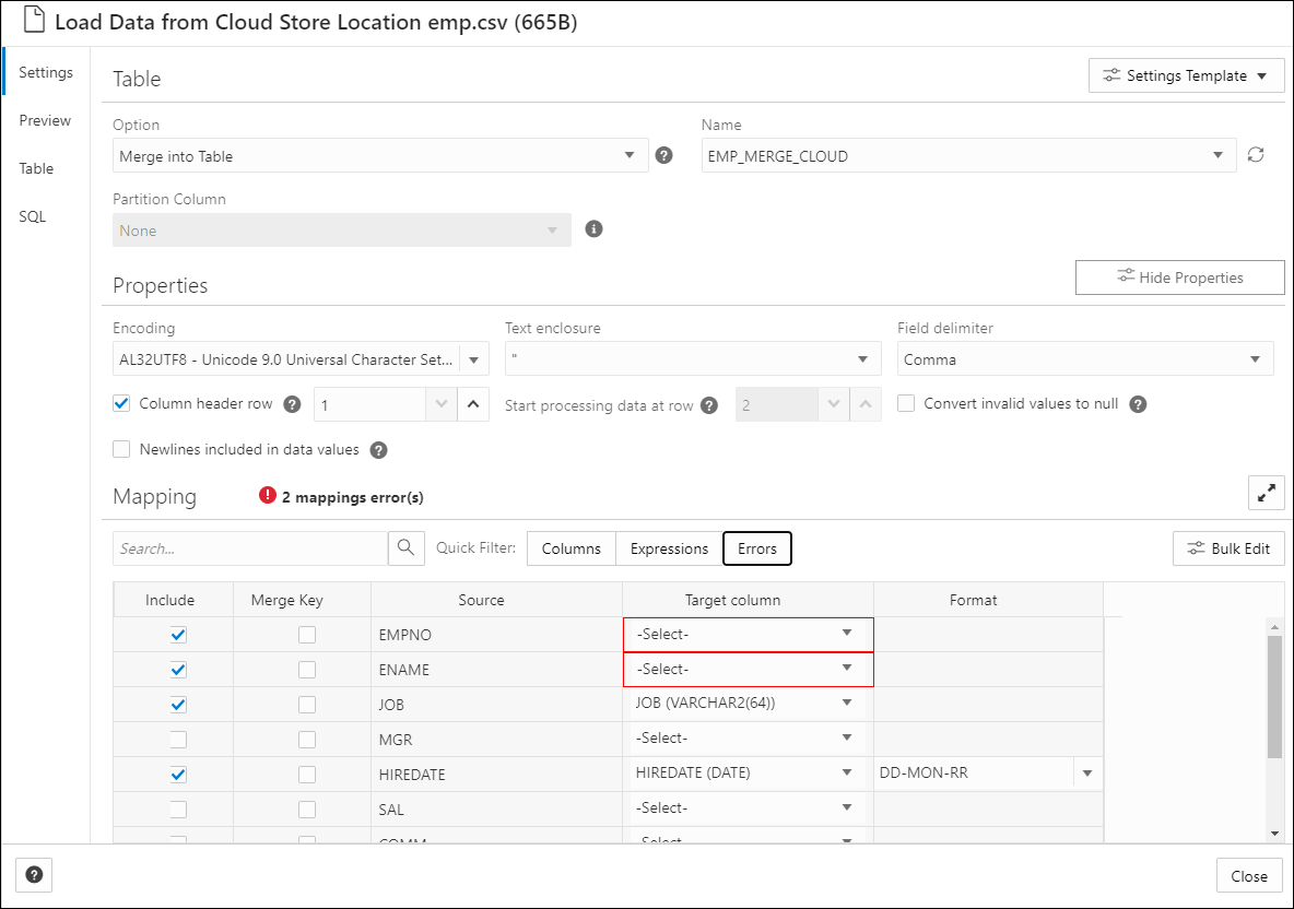
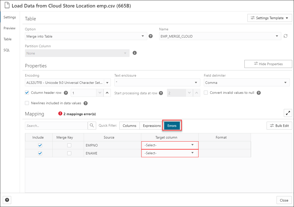
- Load Data from Local Files or Cloud storage: Load the data you wish to analyze into your Oracle Autonomous Database from Local files or Cloud storage. Make sure the data is loaded to the data load cart without any errors. You can view and fix mapping errors from the Errors quick filter in the Load Data from Cloud Store Location. After you load data into the Data load tool,
- Click the Settings icon on the Data Load job cart to review the settings.
- On the Settings pane of the Load Data from Cloud Store Location wizard, if there is a mapping error, the mapping grid cell will be highlighted with red to indicate an invalid value that must be fixed.
- Click the Errors quick filter, it shows only the columns with errors.
- The tools perform sentiment analysis, Key Phrase extraction and Language Detection while you specify settings for the data load job.
Parent topic: Use OCI Language Service Capabilities in Data Studio
Parameters to Analyze Data
When you invoke an Add Expression from the Settings tab, you must configure the model using parameters.
Table 3-3 Parameters for Sentiment Analysis, Key Phase Extraction, and Language Detection
| Parameter | Description |
|---|---|
| Expression Type |
Select any one of the following operations you wish to perform on the input text: Sentiment Analysis, Key Phrase Extraction, and Language Detection. |
| Input Column |
Select the column which you wish to analyze. The input column drop-down only contains columns that Sentiment Analysis, Key Phrase Extraction, and Language Detection support. For Sentiment Analysis, only VARCHAR2, NVARCHAR2, CLOB, or NCLOB target columns will be displayed in the input drop-down. |
| Target Column |
|
Parent topic: Use OCI Language Service Capabilities in Data Studio
Perform Sentiment Analysis
To determine the Sentiments of input data:
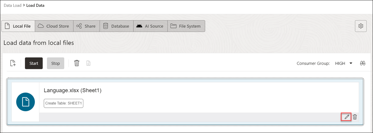
- After you load data into the Data Load cart from local files or cloud storage, you can view the file in the cart. Click the settings icon.
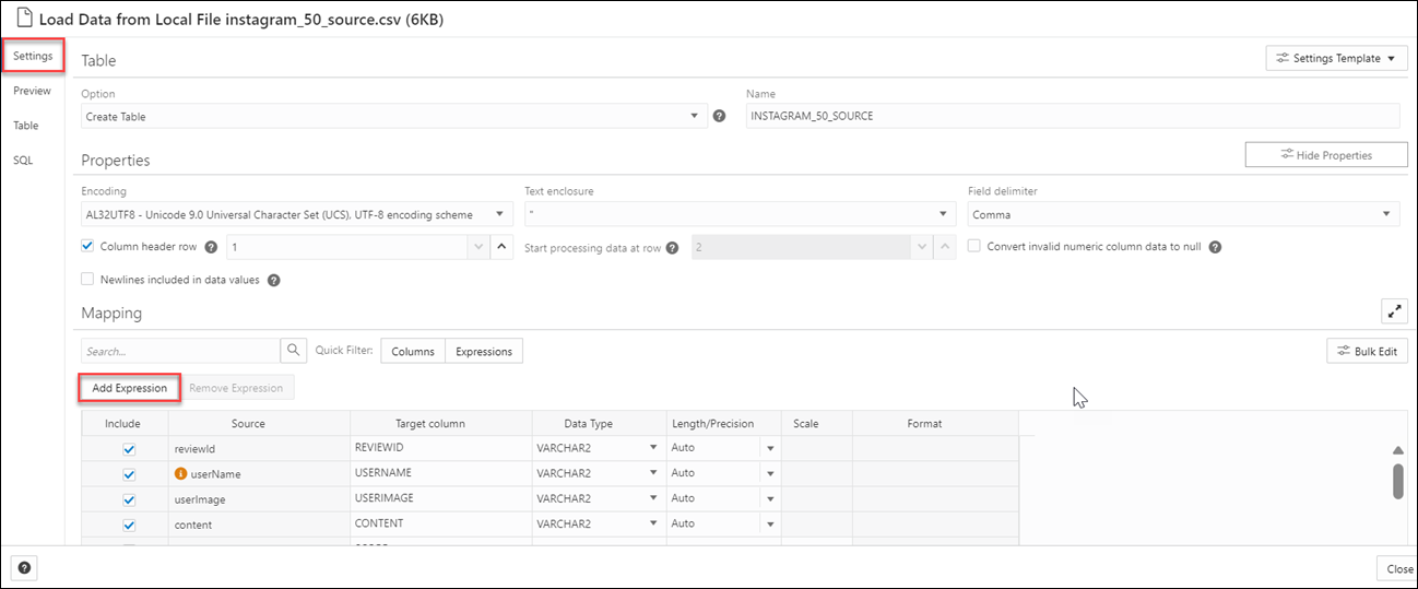
- Clicking the Setting icon opens a Load Data from Local File wizard. In this example, we have loaded data from a local file.
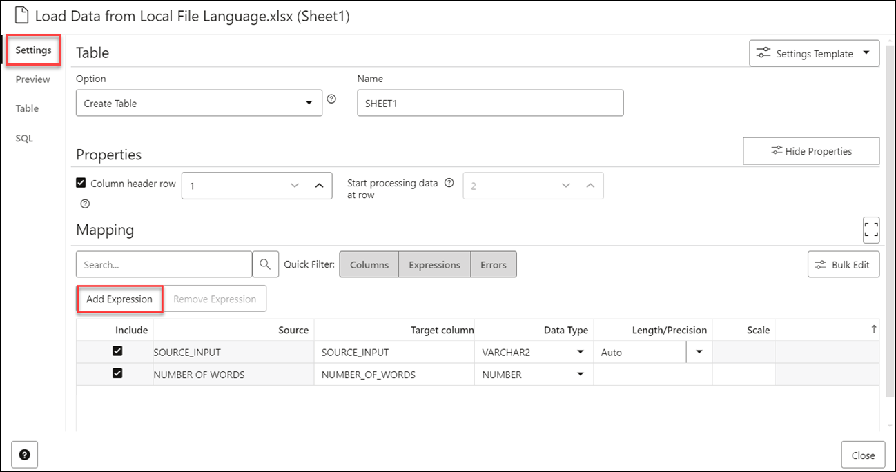
- On the Settings tab of the wizard, click Add Expression under the Mapping section.
This opens the Add Expression dialog box.
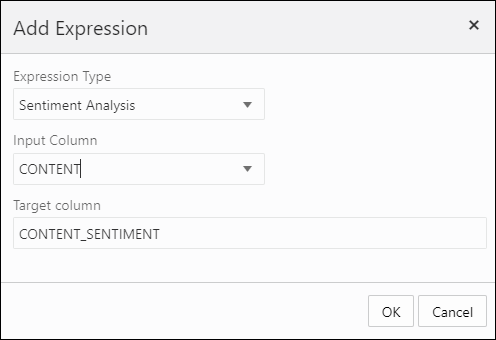
- On the Add Expression dialog, specify the following fields:
- Expression Type: From the Expression Type drop-down, select Sentiment Analysis.
- Input Column: Select the column from the drop-down that you wish to analyze. For example, CONTENT.
- Target column: Enter the name of the newly created expression column. For example, CONTENT_SENTIMENT.
Refer to the Parameters to Analyze Data for more details.
- Click OK. You will see a new row added to the mapping grid. This row determines the output expression column generated by the OCI Language service.
- Click Close.
- Click Start in the Data Load menu cart to load data from local files. You will view a confirmation message asking if you wish to start the load from local files.
- Click Run to confirm.
When the data load job completes, the Table and View Loads of the Data Load page display the details of the source table that is loaded into the tool. It displays the number of rows and columns and when the upload was complete.
- Output Data Generated from OCI Sentiment Analysis
When you analyze columns using OCI Language Service model, the Data Studio generates a new expression column and saves the result in the updated table.
Parent topic: Use OCI Language Service Capabilities in Data Studio
Output Data Generated from OCI Sentiment Analysis
When you analyze columns using OCI Language Service model, the Data Studio generates a new expression column and saves the result in the updated table.
To locate the generated expression column, from the Database Actions Launchpad, navigate to Data Load. Select the table you load under the Table and View Loads section.
Click the three vertical dots beside the load name, and click Table then select View Details.
This opens the Preview tab of the data load which displays the updated source file. For example, here is an output dataset from sentiment analysis of the Instagram application. Here, CONTENT is the target column, and CONTENT_SENTIMENT is the sentiment analysis of the input column. This column displays one of the following values such as positive, neutral, mixed, or negative It displays Null when the tool is unable to determine the sentiment.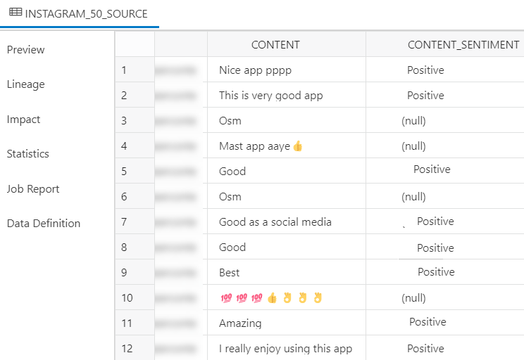
Description of the illustration content-analysis.png
Parent topic: Perform Sentiment Analysis
Perform Key Phrase Extraction
To extract Key Phrase information from input data:
- After you load data into the Data Load cart from local files or cloud storage, you can view the file in the cart. Click the settings icon.
- Clicking the Setting icon opens a Load Data from Local File wizard. In this example, we have loaded data from a local file.
- On the Settings tab of the wizard, click Add Expression under the Mapping section.
This opens the Add Expression dialog box.
- On the Add Expression dialog, specify the following fields:
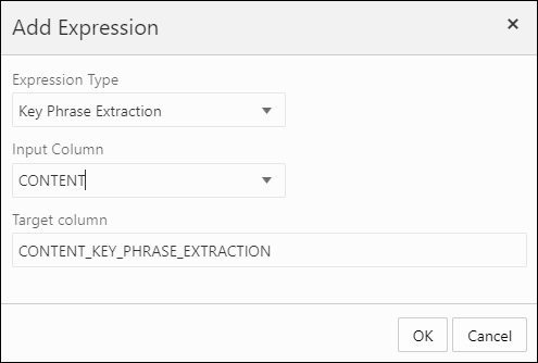
- Expression Type: From the Expression Type drop-down, select Key Phrase Extraction.
- Input Column: Select the column from the drop-down that you wish to analyze. For example, CONTENT.
- Target column: Enter the name of the newly created expression column. For example, CONTENT_KEY_PHRASE_EXTRACTION.
Refer to the Parameters to Analyze Data for more details.
- Click OK. You will see a new row added to the mapping grid .This row determines the output expression column generated by the OCI Language service.
- Click Close.
- Click Start in the Data Load menu cart to load data from local files. You will view a confirmation message asking if you wish to start the load from local files.
- Click Run to confirm.
When the data load job completes, the Table and View Loads of the Data Load page display the details of the source table that is loaded into the tool. It displays the number of rows and columns and when the upload was complete.
- Output Data Generated from OCI Key Phrase Extraction
When you analyze columns using OCI Language Service model, the Data Studio generates a new expression column and saves the result in the updated table.
Parent topic: Use OCI Language Service Capabilities in Data Studio
Output Data Generated from OCI Key Phrase Extraction
When you analyze columns using OCI Language Service model, the Data Studio generates a new expression column and saves the result in the updated table.
To locate the generated expression column, from the Database Actions Launchpad, navigate to Data Load. Select the table you load under the Table and View Loads section.
Click the three vertical dots beside the load name, and click Table then select View Details.
For example, here's an output dataset from sentiment analysis of the Instagram application. Here, CONTENT is the target column, and CONTENT_KEY_PHRASE_EXTRACTION column displays the key phrases extracted from the input column.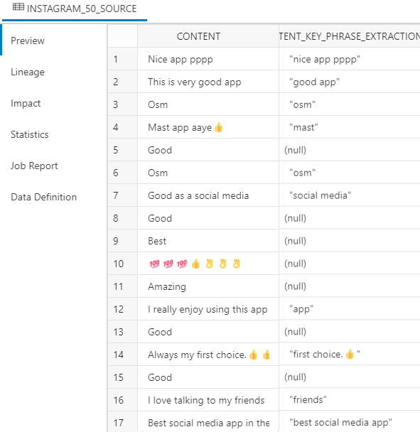
Description of the illustration key-output.png
Parent topic: Perform Key Phrase Extraction
Perform Language Detection
The Data Studio supports the detection of multiple languages.
- After you load data into the Data Load cart from cloud storage, you can view the file in the cart. Click the Settings icon.
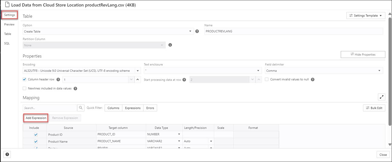
- Clicking the Setting icon opens a Load Data from Cloud Store Location wizard.
- On the Settings tab of the wizard, click Add Expression under the Mapping section.
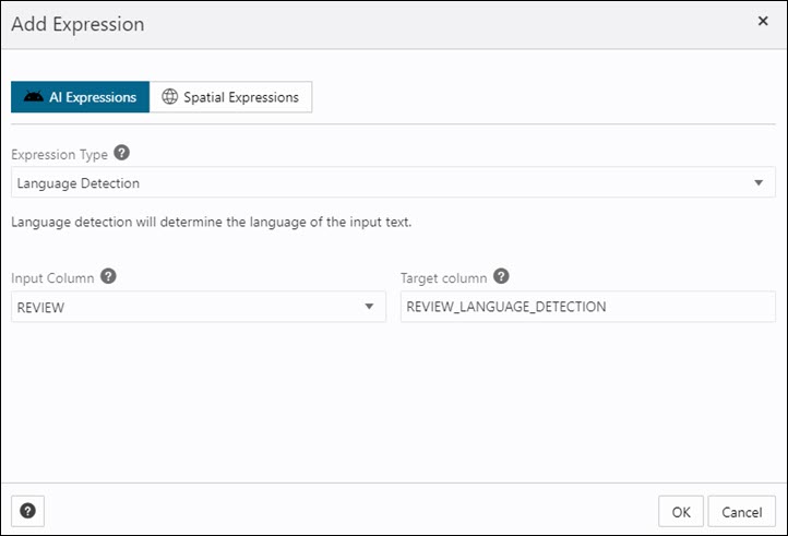
This opens the Add Expression dialog box. Select AI Expressions.
Description of the illustration add-expn-lang.bmp - On the Add Expression dialog, specify the following fields:
- Expression Type: From the Expression Type drop-down, select Language Detection.
- Input Column: Select the column from the drop-down that you wish to analyze. In this case, we need to detect the language of the Review column. For example, REVIEW.
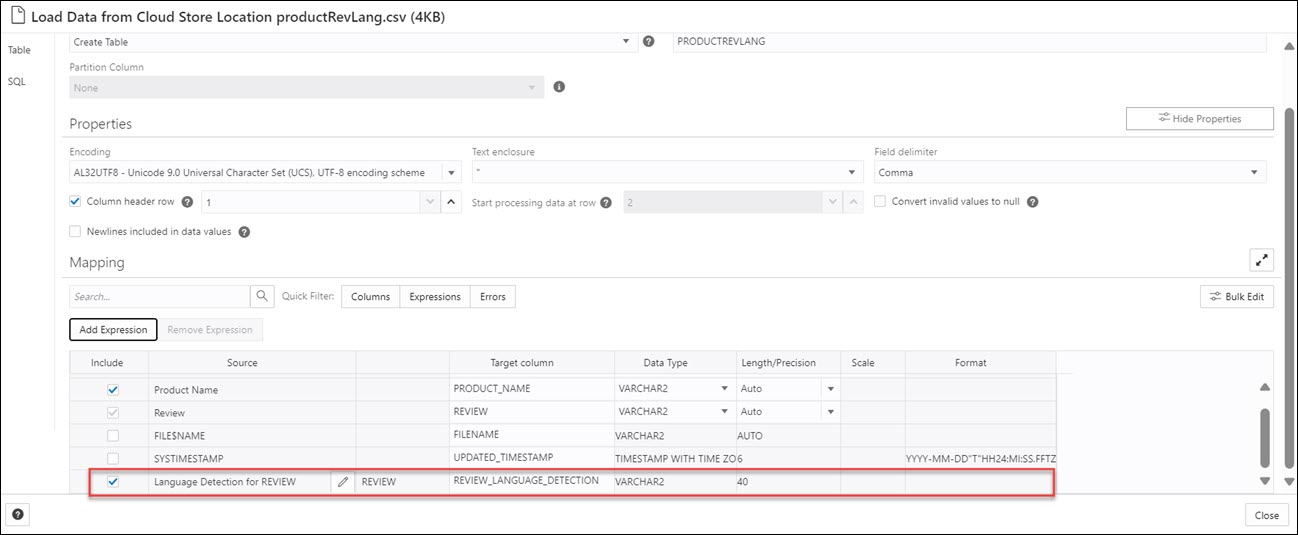
- Target column: Enter the name of the newly created expression column. For example, REVIEW_LANGUAGE_DETECTION.
Refer to the Parameters to Analyze Data for more details.
- Click OK. You will see a new row added to the mapping grid .This row determines the output expression column generated by the OCI Language service.
- Click Close.
- Click Start in the Data Load menu cart to load data from local files. You will view a confirmation message asking if you wish to start the load from local files.
- Click Run to confirm.
When the data load job completes, the Table and View Loads of the Data Load page display the details of the source table that is loaded into the tool. It displays the number of rows and columns and when the upload was complete.
- Output Data Generated from OCI Language Detection
When you analyze columns using OCI Language Service model, the Data Studio generates a new expression column and saves the result in the updated table.
Parent topic: Use OCI Language Service Capabilities in Data Studio
Output Data Generated from OCI Language Detection
When you analyze columns using OCI Language Service model, the Data Studio generates a new expression column and saves the result in the updated table.
To locate the generated expression column, from the Database Actions Launchpad, navigate to Data Load. Select the table you load under the Table and View Loads section.
Click the three vertical dots beside the load name, and click Table then select View Details.
For example, here's an output dataset from language detection of the Review column. Here, REVIEW is the target column, and REVIEW_LANGUAGE_DETECTION column displays the language detected from the input column.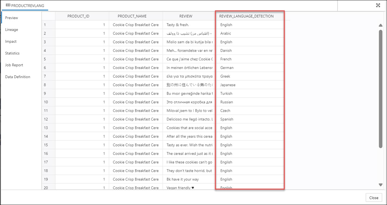
Description of the illustration output-language.bmp
Parent topic: Perform Language Detection
Perform Text Translation
The Data Studio supports the translation of multiple languages supported by OCI Language Service.
To determine the translated input text:
- After you load data into the Data Load cart from local files, you can view the file in the cart. Click the settings icon.
- Clicking the Setting icon opens a Load Data from Local File wizard.
- On the Settings tab of the wizard, click Add Expression under the Mapping section.
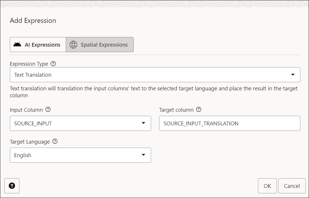
This opens the Add Expression dialog box. Select AI Expressions.
- On the Add Expression dialog, specify the following fields:
- Expression Type: From the Expression Type drop-down, select Text Translation.
- Input Column: Select the column from the drop-down that you wish to analyze. In this case, we need to translate the text of the SOURCE_INPUT column.
- Target column: Enter the name of the newly created expression column. For example, SOURCE_INPUT_TRANSLATION.
- Target Language: Select the language of the text the tool translates from the drop-down. For example, English.
Refer to the Parameters to Analyze Data for more details.
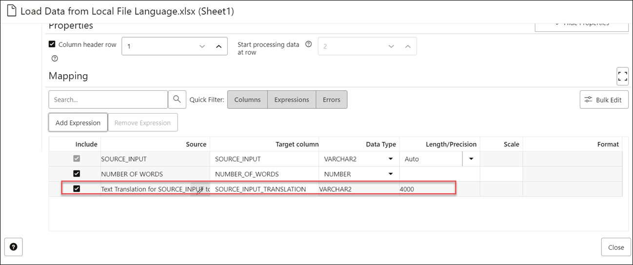
- Click OK. You will see a new row added to the mapping grid .This row determines the output expression column generated by the OCI Language service.
- Click Close.
- Click Start in the Data Load menu cart to load data from local files. You will view a confirmation message asking if you wish to start the load from local files.
- Click Run to confirm.
When the data load job completes, the Table and View Loads of the Data Load page display the details of the source table that is loaded into the tool. It displays the number of rows and columns and when the upload was complete.
- Output Data Generated from OCI Text Translation
When you analyze columns using OCI Language Service model, the Data Studio generates a new expression column and saves the result in the updated table.
Parent topic: Use OCI Language Service Capabilities in Data Studio
Output Data Generated from OCI Text Translation
When you analyze columns using OCI Language Service model, the Data Studio generates a new expression column and saves the result in the updated table.
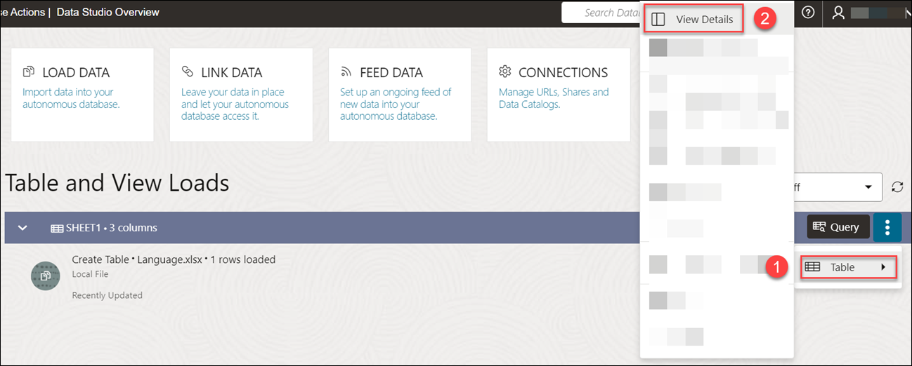
To locate the generated expression column, from the Database Actions Launchpad, navigate to Data Load. Select the table you load under the Table and View Loads section.
Click the three vertical dots beside the load name, and click Table then select View Details.
Parent topic: Perform Text Translation
Use OCI Document Understanding to extract Tables from Images
You can utilize Oracle Cloud Infrastructure(OCI) Document Understanding Capabilities such as Table Extraction to detect tables from the data you load.
The supported file formats to use this feature are PDF, JPEG, JPG, PNG and Tag Image File Format (TIFF) formats.
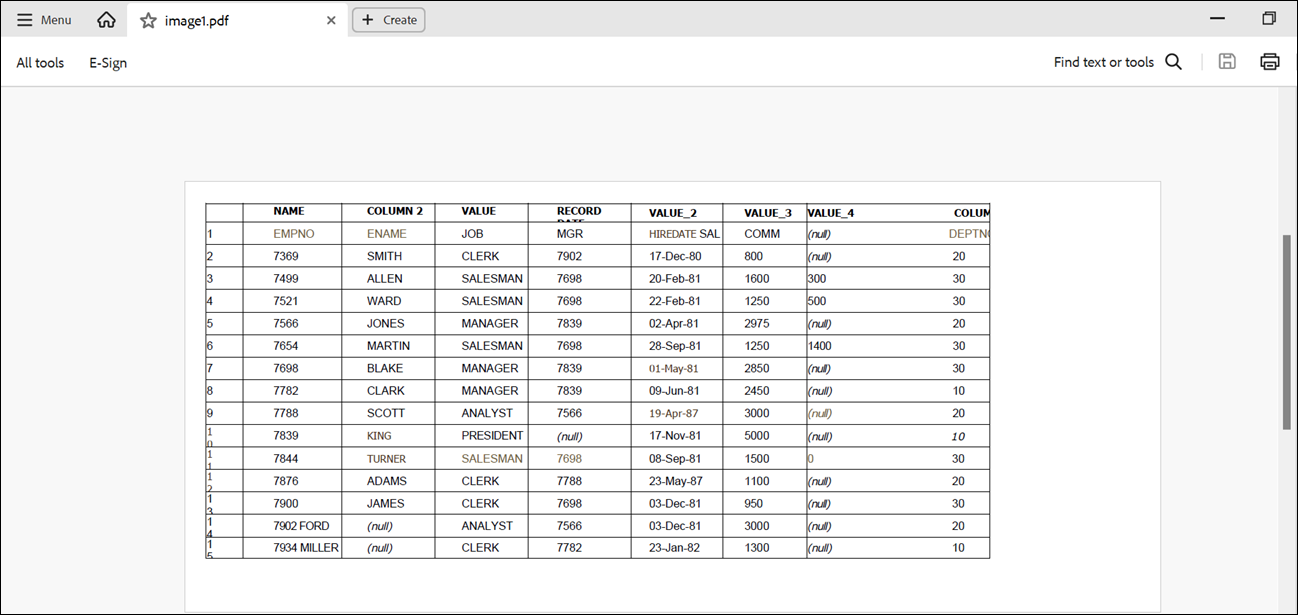
For example, if a PDF document consists of all the employee details including their hiring date and salary, document understanding will identify the table and extract the table structure. It will extract the content of the table while maintaining the row and column relationship of cells.
- Overview of Table Extraction
The Load Data tool supports Table Extraction in loading data from local files and loading data from cloud storage. - Perform Table Extraction from Image
Let us perform table extraction with a sample PDF.
Parent topic: Loading Data
Overview of Table Extraction
The Load Data tool supports Table Extraction in loading data from local files and loading data from cloud storage.
Table Extraction
OCI Document Understanding service allows customers to uncover insights in unstructured documents powered by deep learning models. It enables you to extract text, tables and identify document types among other great capabilities. Table Extraction identifies all the tables in a document and extracts the content in tabular format maintaining the row/column relationship.
This service is available for source data in English Language only.
For more details, see Table Extraction.
Perform Table Extraction from Image
Let us perform table extraction with a sample PDF.
You can see a table in the PDF below.
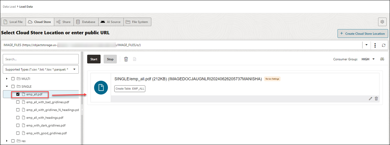
- Load the PDF file into the Data Load cart from the cloud storage. You can drag and drop the file from the navigator to the cart.
- Click Start to load the data. You will receive a notification that confirms if you wish to start loading the data. Click Run to continue.
- After the loading is complete, you can view the loaded file under Table and View Loads in the Data Load dashboard.
- Extract the table from the PDF you loaded in the autonomous database:
- Click Database Actions in the breadcrumb.
- Select Development, then click SQL.
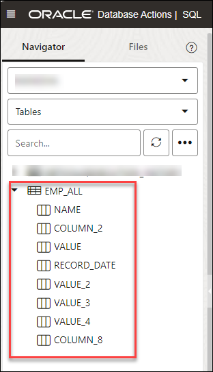
- Select Tables, on the left Navigator, from the object drop-down. From the list of available tables, drag and drop the
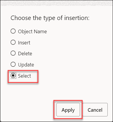
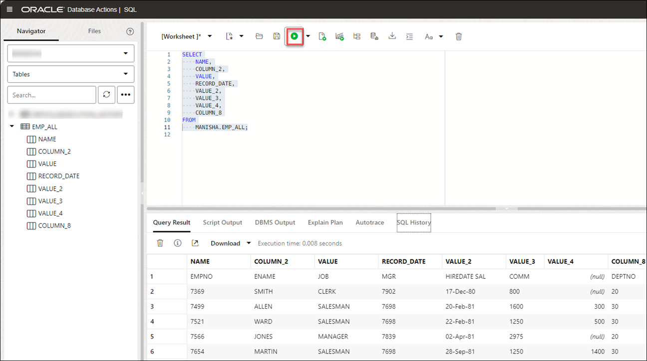
EMP_ALLtable to the worksheet.A dialog displays offering the types of available insertions.
Click Select, then Apply.
- Click Run (the arrow icon at the top of the worksheet). The tool displays the extracted table under the Query Results tab.
Use GeoJSON in Data Load
A GeoJSON object accommodates information about the specific geometry (e.g. Point, Line, Polygon, etc.) along with optional metadata (e.g. ID, etc.).
The extension for a GeoJSON file is *.geojson. You can load GeoJSON data into the Autonomous Database using the Data Load in Data Studio. If the table contains GeoJSON data, then the data is loaded in a column that projects GeoJSON data from the document set of SQL data type SDO_GEOMETRY.
Load a table with GeoJSON Data
When you load a table in Data Studio with GeoJSON data and review its settings, you will see that it creates table Brazil_Geo, which has a column geometry of GeoJSON data.
After you load BRAZIL_GEO you will view that the tool loads GeoJSON object into a new column geometry with the data type SDO_GEOMETRY.
Description of the illustration edittable-geo.png
You can also view the same in the Data Definition tab when you View Details of the Table load after it is run.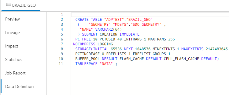
Description of the illustration datadefinition-geo.png
- Add Spatial Expression for GeoJSON columns
Oracle Spatial is designed to make spatial data management easier and more natural to users of location-enabled applications and geographic information system (GIS) applications. - Parameters for Spatial Data Analysis
When you invoke an Add Expression and select Spatial Expressions from the Add Expression wizard, you must configure the model using parameters. - Perform Spatial Analysis
You can load Spatial data using the Data Load tool from local files or cloud storage. - Output Data Generated from Spatial Analysis
When you analyze columns using Spatial Expressions, the Data Studio generates a new expression column and saves the result in the updated table.
Parent topic: Loading Data
Add Spatial Expression for GeoJSON columns
Oracle Spatial is designed to make spatial data management easier and more natural to users of location-enabled applications and geographic information system (GIS) applications.
Once spatial data is stored in an Oracle database, it can be easily manipulated, retrieved, and related to all other data stored in the database.
The spatial data model in Oracle Spatial is a hierarchical structure consisting of elements, geometries, and layers. Layers are composed of geometries, which in turn are made up of elements.
Tolerance is used to associate a level of precision with spatial data. Tolerance reflects the distance that two points can be apart and still be considered the same (for example, to accommodate rounding errors). The tolerance value must be a positive number greater than zero. See Tolerance in Spatial Data for more information.
Parent topic: Use GeoJSON in Data Load
Parameters for Spatial Data Analysis
When you invoke an Add Expression and select Spatial Expressions from the Add Expression wizard, you must configure the model using parameters.
Table 3-4 Parameters for Spatial Data Analysis
| Parameter | Description |
|---|---|
| Expression Type |
Select any one of the following spatial attributes such as Length or Area:
|
| Input Column |
Select the column which you wish to analyze for Spatial Data: You will by default view a |
| Target Column |
This is the newly created expression column defined in the target table which stores the result of the Spatial Expression and depends on the expression type value you select:
|
Parent topic: Use GeoJSON in Data Load
Perform Spatial Analysis
You can load Spatial data using the Data Load tool from local files or cloud storage.
- After you load data into the Data Load cart from local files or cloud storage, you can view the file in the cart. Click the Settings icon.
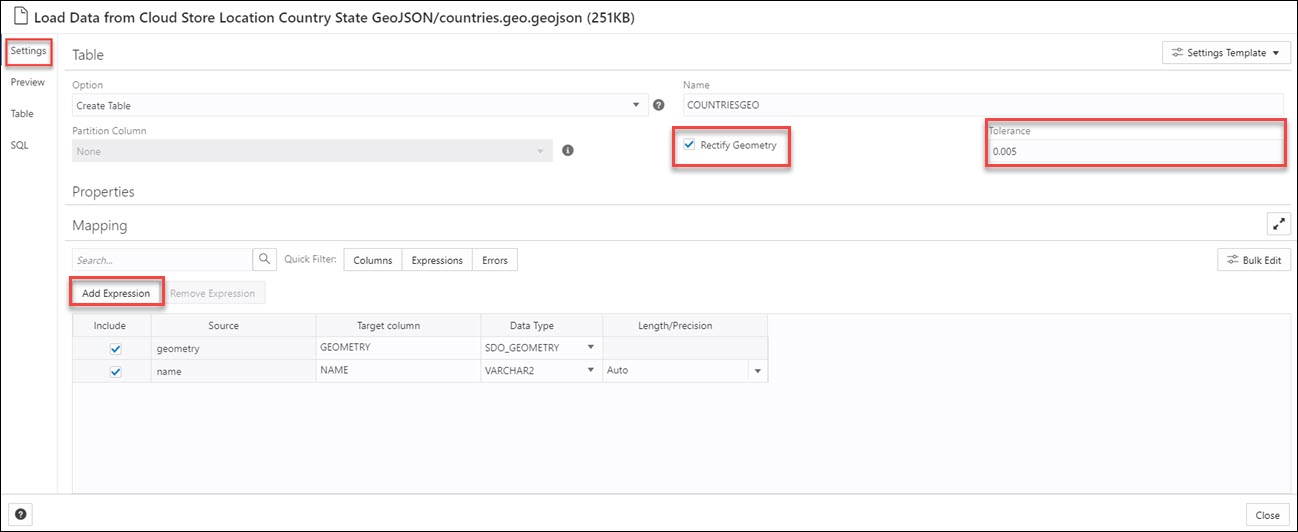
- On the Settings tab of the wizard, select Rectify Geometry to fix invalid geometries. This icon corrects the most common errors such as duplicate points, polygon orientation errors, polygon construction errors etc. If it detects any uncorrectable error, it fails with an
ORA-13199: the given geometry cannot be rectifiedexception.Note
You cannot fix geometries having wrong orientation with the. Rectify Geometry icon. - Specify the Tolerance value. In the above example, we specify 0.005 as tolerance, i.e., 5mm.
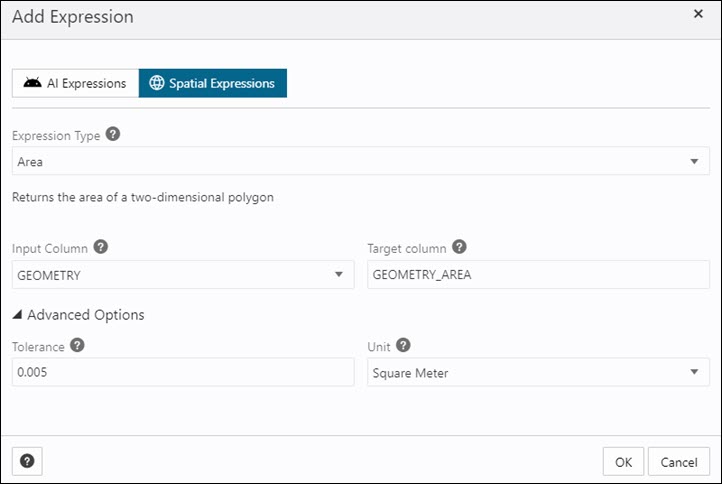
- Click Add Expression under the Mapping section and select Spatial Expressions.On the Add Expression dialog, specify the following fields:
- Expression Type: From the Expression Type drop-down, select Area to display the area of a two-dimensional polygon. You can also select Length to display the perimeter of a two-dimensional polygon.
- Input Column: You will view a
GEOMETRYcolumn by default. This source column stores the area of the geometry. In case you select Length as an expression type, this source column stores the length of the geometry. - Target column: Specifies the name of the newly created special expression column. For example,
GEOMETRY_AREAfor Area type expression parameter andGEOMETRY_LENGTHfor Length type expression parameter.
Under the Advanced Options section, specify the following field values:- Tolerance: Enter the tolerance value. For example,
0.005. - Unit: Select a unit of measure of the tolerance from the drop-down. For example,
Square meter.
Note
If the file you load does not contain spatial data, you will view the following error on the Add Expression wizard "No input columns have the SDO_GEOMETRY data type for the currently selected expression type of Area".Refer to the Parameters for Spatial Data Analysis for more details.
- Click OK. You will see a new row added to the mapping grid. This row determines the output spatial expression column generated by the OCI Language service. In this example, you can view a new
GEOMETRY_AREAwill be created in the target table after we load the table.
For more information on Oracle Spatial, refer to Oracle Spatial Developer's Guide.
When the data load job completes, the Table and View Loads of the Data Load page display the details of the source table that is loaded into the tool. It displays the number of rows and columns and when the upload was complete.
Parent topic: Use GeoJSON in Data Load
Output Data Generated from Spatial Analysis
When you analyze columns using Spatial Expressions, the Data Studio generates a new expression column and saves the result in the updated table.
To locate the generated expression column, from the Database Actions Launchpad, navigate to Data Load. Select the table you load under the Table and View Loads section.
Click the three vertical dots beside the load name, and click Table then select View Details.
This opens the Preview tab of the data load which displays the updated source file. For example, here is an output dataset from spatial analysis of the COUNTRIESGEO.GeoJSON file. Here, GEOMETRY_AREA is the spatial analysis of the input column. This column displays the area of the two-dimensional polygons.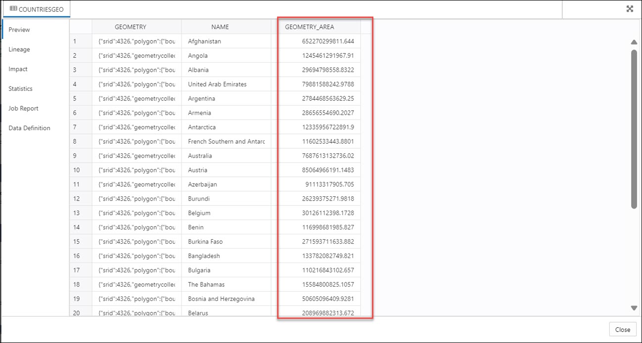
Description of the illustration spatial-output.bmp
Parent topic: Use GeoJSON in Data Load
Load Apache Iceberg Tables
Data Studio supports loading and linking Iceberg tables from the object store.
The tool can load multiple versions of the same file.
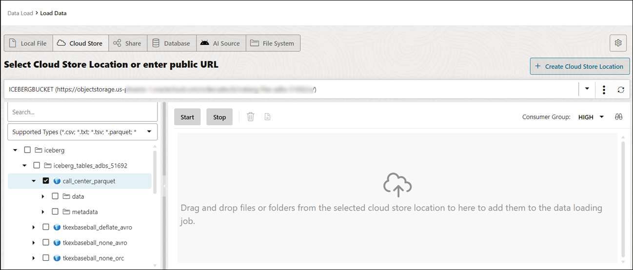
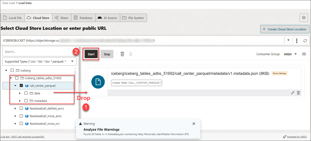
- Select the Cloud Store Location that has iceberg tables defined. In this example, we will select the
ICEBERGBUCKETstored in OCI.You can detect the Iceberg files with the Iceberg symbol

Description of the illustration symbol.png
beside its name. - Drag the folder to the file navigator on the left and drop it into the cart on the right. The folder also consists of the metadata JSON file that keeps track of the table snapshots, partitioning scheme, and schema information.
When you add the folder to the cart, a warning about the number of files consisting of a Personal Identifiable Information (PII) prompt is displayed.
Note
: If you load multiple files instead of a folder, the tool asks if you want to load all the objects from the multiple source files into a single target table. Click OK to continue or Escape to cancel. - Click Start in the data link cart menu bar. You will view a notification that says if you wish to start the load from the cloud store. Select Run to continue.
- You will view the loading progress under Table and View Loads. After loading, you will view the Report and Reload icons on the table load.
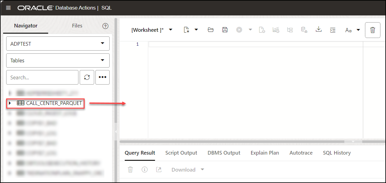
- Query Iceberg tables you loaded in the Autonomous Database:
- Click Database Actions in the breadcrumb.
- Select Development, then click SQL.
- Select Tables, on the left Navigator, from the object drop-down. From the list of available views, drag and drop the CALL_CENTER_PARQUET table to the worksheet.
- A dialog displays offering the types of available insertions.
Click Select, then Apply.
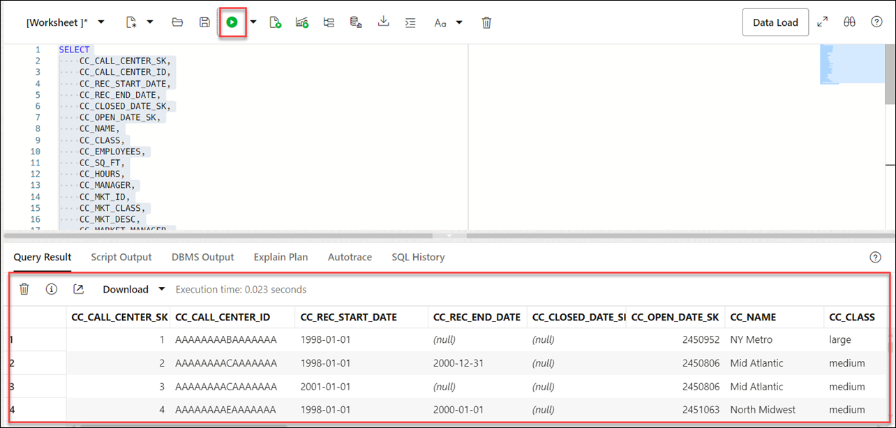
- Click Run (the arrow icon at the top of the worksheet). The tool displays the iceberg data under Query Results.
Parent topic: Loading Data
Loading Data from File System
You can load files from file system directories to your Autonomous Database.
You can set filters on the data for a table to load only the specified data. For example, to limit the files to only those that are CSV files, enter *.CSV in the file extension filter.
- On the Data Studio tab and select Data Load. You will view the Data Load dashboard.
- Click LOAD DATA and select the File System option.
On the top of the page you need to select the directory from where you need to load the files. On the left side of the page is a navigator pane, where you choose the files in the directory containing the data. On the right of the page is the data load cart, where you stage the files and folders for the data load job. You can set options for the data load job before running it. The Autonomous Database comes with predefined CPU/IO shares assigned to different consumer groups. You can set the consumer group to either low, medium or high while executing a data load job depending on your workload. To load files from a directory into your database, do the following:
- Prepare the Data Load Job: Refer to the Prepare the Data Load Job section for more details.
- Add Files or Folders for the Data Load Job: Refer to the Add Files or Folders for the Data Load Job section for more details.
- Enter Details for the Data Load Job: Refer to the Enter Details for the Data Load Job for more details.
- Run the Data Load Job: Refer to the Run the Data Load Job section for more details.
- View Details About the Data Load Job After It Is Run: Refer to the View Details About the Data Load Job After It Is Run section for more details.
- View the Table Resulting from the Data Load Job: Refer to the View the Table Resulting from the Data Load Job section for more details.
- Create Directories in Database Actions
In the Autonomous Database, there is a preconfigureddata_pump_dirwhere you can store files. You can also create directories, drop directories, and attach network file systems.
Parent topic: Loading Data
Create Directories in Database Actions
In the Autonomous Database, there is a preconfigured data_pump_dir where you can store files. You can also create directories, drop directories, and attach network file systems.
For example, you can use the CREATE DIRECTORY command to create additional directories. Use the database DROP DIRECTORY command to drop directories and use DBMS_CLOUD.LIST_FILES to list the contents of a directory.
Create a Directory
To add a directory, you must have the CREATE ANY DIRECTORY system privilege. The ADMIN user is granted the CREATE ANY DIRECTORY system privilege. The ADMIN user can grant CREATE ANY DIRECTORY system privileges to other users.
See CREATE DIRECTORY for more information.
CREATE DIRECTORYcreates the database directory object in the database and also creates the file system directory. For example the directory path could be:/u03/dbfs/7C149E35BB1000A45FD/data/stage-
You can create a directory in the root file system to see all the files with the following commands:
CREATE OR REPLACE DIRECTORY ROOT_DIR AS '';After you create the
ROOT_DIRdirectory, use the following command to list all files:SELECT * FROM DBMS_CLOUD.list_files('ROOT_DIR'); -
To run
DBMS_CLOUD.LIST_FILESwith a user other than ADMIN you need to grant read privileges on the directory to that user.
Let us demonstrate how to create a directory and access it from Data Studio:
- Create a directory in Database Actions:
Login to your Database Actions instance and select the SQL card under Development. You can view the SQL worksheet. Now create a directory and attach a file system name of your choice to the directory you create. In the below given example,
FSS_DIRis the name of the directory.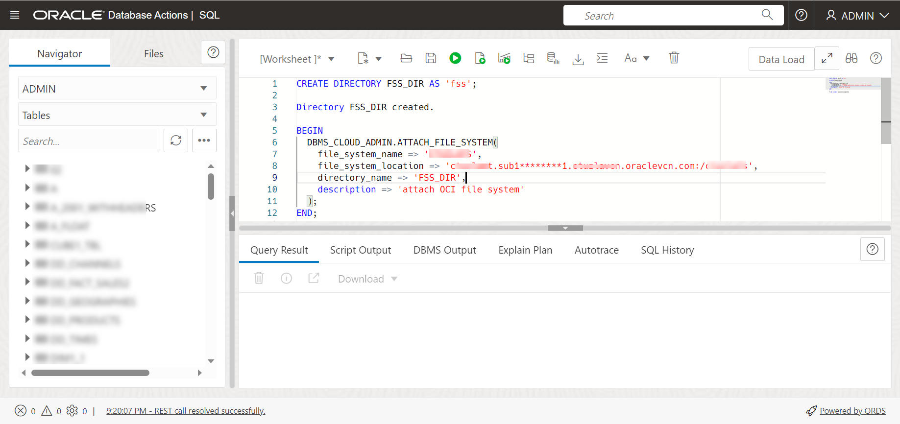
Description of the illustration create-directory.pngRun the above command. The above command gives the following output:
PL/SQL procedure successfully completed.
- Attach the file systemAttach your file system with the name of your choice to the
FSS_DIRdirectory via the DBMS_CLOUD_ADMIN.ATTACH_FILE_SYSTEM procedure.BEGIN DBMS_CLOUD_ADMIN.ATTACH_FILE_SYSTEM( file_system_name => '********', file_system_location => '*******.sub1********1.********.oraclevcn.com:/********', directory_name => 'FSS_DIR', description => 'attach OCI file system' ); END; /Run the above command to view the following output:
PL/SQL procedure successfully completed. - To view the attached file system, run the following command:
SELECT file_system_name, file_system_location, directory_path FROM
        dba_cloud_file_systems;
You will view the file system name, file system location and directory path.
- You can view the new directory along with the files attached to it by navigating to Load Cloud Object under Data Load menu of the Data Studio tool. Click the Select Cloud Store location drop-down.
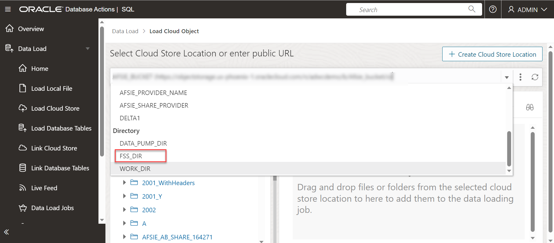
Description of the illustration new-dir.png
You can view the newly created directory FSS_DIR. You can load data from the file system directories to the autonomous database using the Data Load tool. See Loading Data from File System.
Parent topic: Loading Data from File System
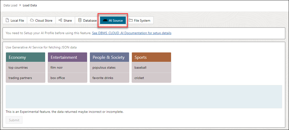
Loading Data from AI Source
You can use Data Studio tools to load data from AI source.
On the Data Load dashboard, click Load Data card, and select AI Source.
You need to perform a pre-requisite of setting up your AI profile before using this feature. See Configure DBMS_CLOUD_AI Package for details on the setup of this feature.
- An OpenAI account, or a Cohere account, or Azure OpenAI service
- An access to
DBMS_CLOUD_AIpackage.
Follow the steps in Use DBMS_CLOUD_AI to Configure AI Profiles section to create and configure your AI profile and utilize this feature.
Parent topic: Loading Data
Loading Data from Share
You can select tables from a Share. You need to subscribe and access provided data share.
To load tables from a share, click Load Data on the Data Load Dashboard. Click Share on the Load Data page. Click + Subscribe to Share Provider to subscribe to a Share Provider.
Subscribe to the Data Share Provider
- On the Subscribe to Data Share Provider, enter the Provider Name.
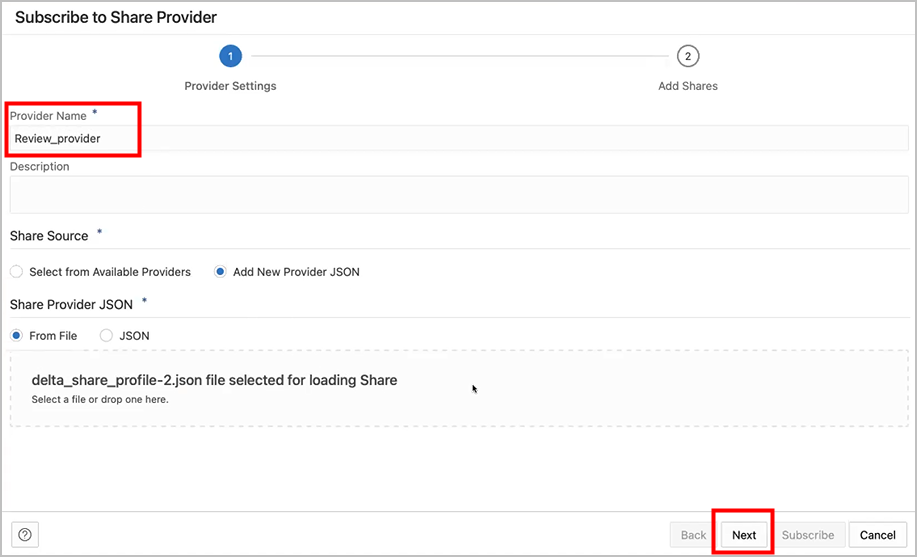
Description of the illustration subscribe_1.png - Select Add New Provider JSON and click on the Delta Share Profile JSON to drag and drop the JSON profile.
- Click Next to progress to the Add Shares tab.
- Select the level of network access you want to allow from your database to the host with the Share REST endpoint, and click Run. In this example, Allow access to Host Only is selected.
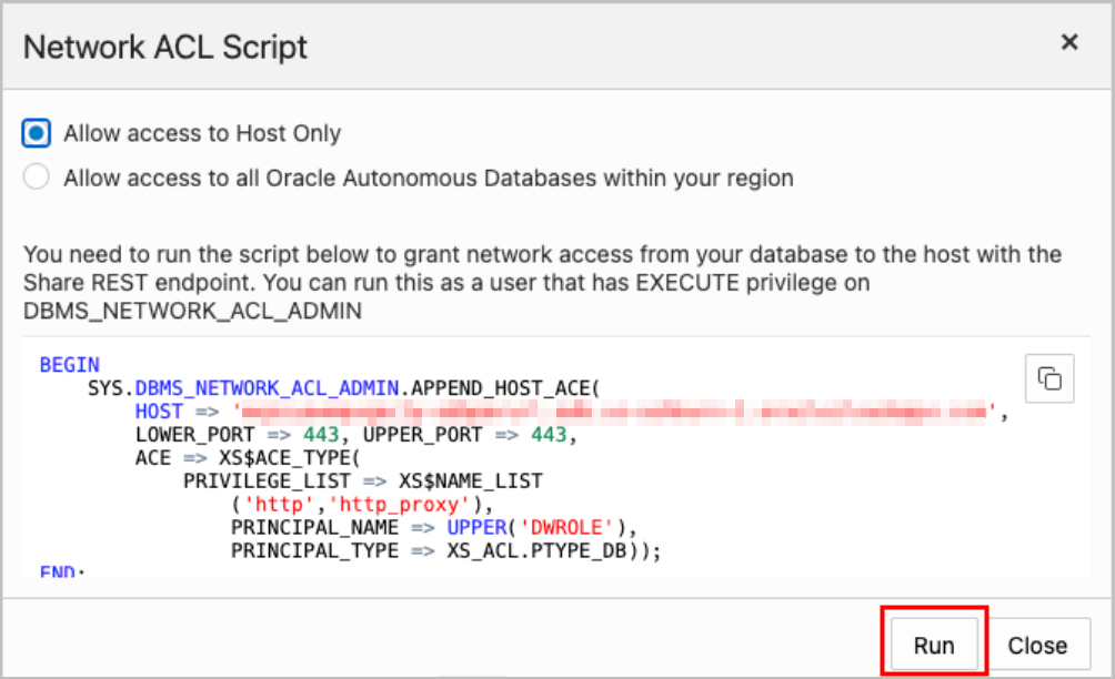
Description of the illustration network_acl_script.png - To register the shares available to you, move shares from Available Shares to Selected Shares and click Subscribe.
The screenshot below shows the REVIEWS share moved from Available Shares to Selected Shares before clicking Subscribe.
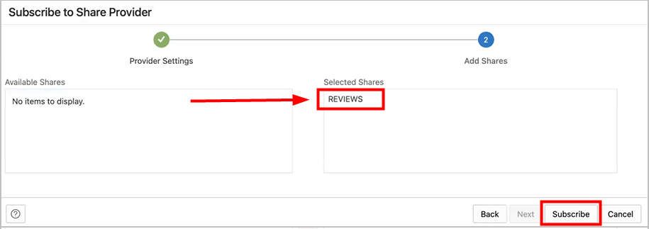
Description of the illustration subscribe_2.png - Create external tables derived from tables selected from the data share.
- Drag and drop tables from the selected share. You can optionally click settings to view the table details.
In this example, the only table selected is HOTEL_REVIEWS.

Description of the illustration sel_tbls.png - You can optionally change the name of your table and click Close.
In this example, the name is changed from HOTEL_REVIEWS to HOTEL_REVIEWS_SHARE.
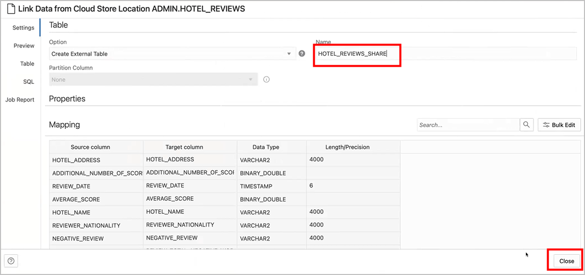
Description of the illustration name_change.png - Create the external table by clicking Start, on the Select Share page, and then clicking Run on the Run Data Load Job dialog.

Description of the illustration start_run.png - When the external tables are created the Complete message is displayed.

Description of the illustration xt_complete.png - Click on the external table name to view the table details.
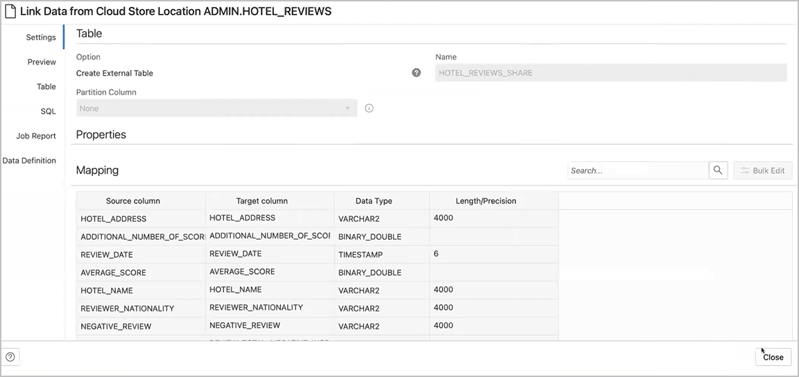
Description of the illustration xt_details.png
- Drag and drop tables from the selected share. You can optionally click settings to view the table details.
- View the created tables from Database Actions.
- Click on Database Actions, in the breadcrumb, to go back to the Database Actions launchpad.
- Click on the SQL tile.
- Select the external table, drag and drop it into the worksheet.
The SQL Select statement for the table appears. This SQL statement can be run to consume the shared data.
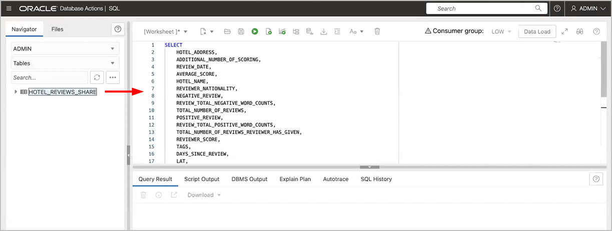
Description of the illustration xt_sql.png
- Drag and drop tables from selected share
Parent topic: Loading Data
Create Live Feed from Data Load
The Data load tool loads the data from folders in cloud object stores and enables it to schedule repeated data loads in real time. This is the creation of Live Feed from a data load job.
Once the data load is complete, you can create a Live Feed from a cart item that loaded an object store folder using the Create Table or Drop Table and Create New Table options.
- Click Selector to display the navigation menu. Under Data Studio, select Data Load.
- Select the Load Data tile to load data from various sources such as local files, databases, cloud store, directories, and Shares.
- Click Cloud Storesto load objects from URLs or Cloud store links.
- Select the cloud store location from the drop-down. If are not able to view the cloud store location, select Create Cloud Store Location to create a new cloud store location. Follow the steps described in the Create Oracle Cloud Infrastructure Native Credentials if you do not have a cloud location available.
- After you select the cloud store location, you can view the list of folders and files present in the cloud storage. Add files from the cloud store to the data load cart, where you can edit the details of the load job.
Note
The Data load tool does not support the creation of a live feed from a loaded cart item that consists of a single file in CSV, XLS, XLSX, TSV, TXT, XML, JSON, and AVRO format or of a folder that contains a file in XLSX format. - To add the folders, drag a folder from the file navigator on the left and drop them into the cart on the right. When you add the folder to the cart, a prompt is displayed that asks if you want to load all the objects from the multiple source files into a single target table. Click Yes to continue or No to cancel. You can add multiple folders to the cart, the data represented by each card will be loaded into a separate table, but all the items in the cart will be processed as part of the same data load job.
- Select Settings (pencil icon) from the data load cart to enter the details about the data load job.
- In the Settings tab of the Load Data from the Cloud Store Location, you can select Create Table or Drop Table and Create New Table from the Option drop-down.
Note
The Live feed tool works with the Data load job only if you create a table and insert the data into a new table or drop the existing table and insert the data into a new table. - Enter the other details for the data load job. For more information on entering the details, refer to the Enter Details for the Data Load Job topic.
- Once you have added data sources to the data load cart and entered details about the data load job, select Start to run the job.
- After the data load job is run, the data load cart displays a green check mark
which indicates that the data load job is complete. - Click Create Live Table Feed on the data load cart to create a Live table feed from the data load job. You will view a successful message that says the creation of Live Table feed is successful and if you wish to edit the live table feed. Click Yes to continue and No to cancel. Selecting Yes opens an Edit Live Table Feed wizard.
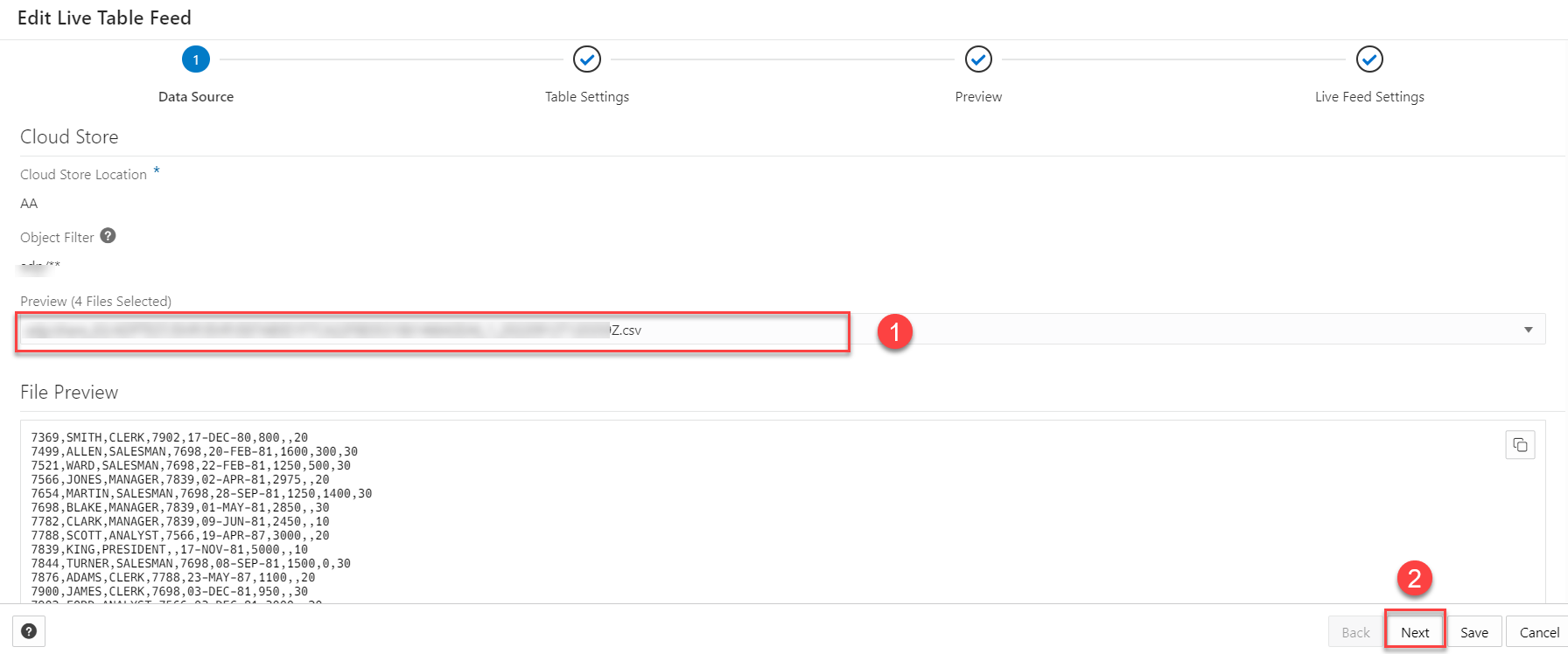
- On the Edit Live Table Feed wizard, you can view the Cloud Store Location of the source folder and the Object Filter applied to the data.
Select any file whose data you want to preview from the Preview drop-down in the Data Source tab: The field shows the total number of files present in the cloud store folder you loaded. A preview of the data is displayed.
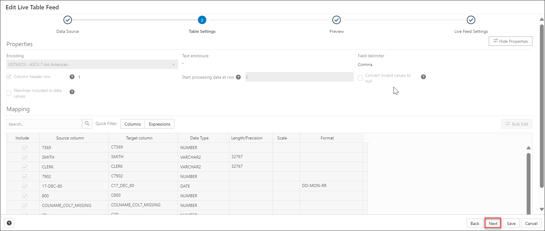
- Click Next to progress to the Table Settings tab.You can view the Properties and Mapping details of the data load job on the Table Settings tab.Note
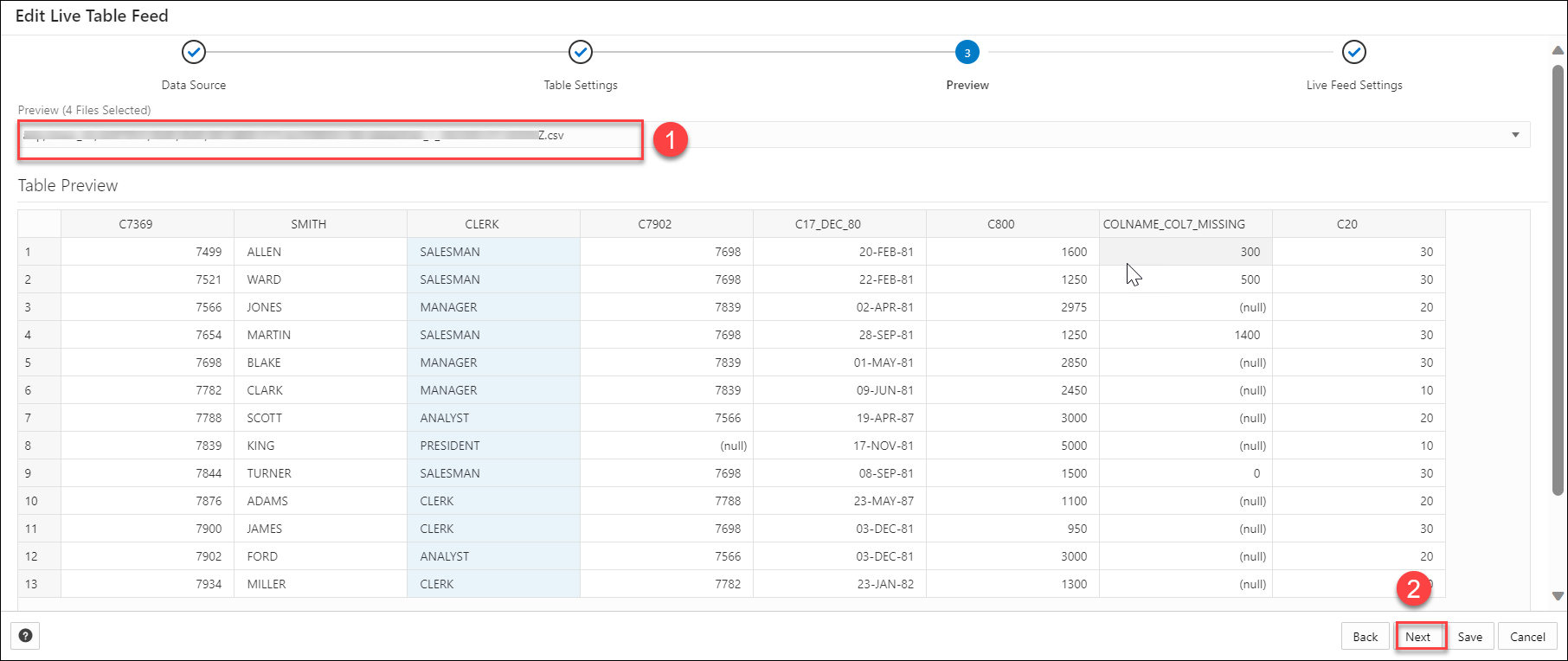
You cannot select or edit any of the details of this tab. - Click Next to progress to the Preview tab of the wizard.
Select any file from the Preview drop-down to view the file. The Table Preview displays the preview of the file you select from the drop-down.
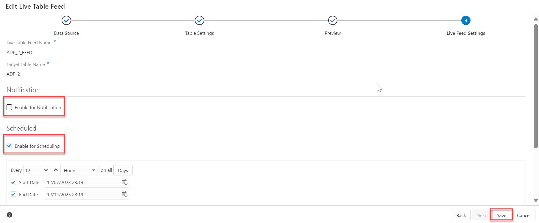
- Click Next to view the Live Feed Settings tab of the wizard. On the Live Feed Settings tab, specify the following values in the field:
-
Enable for Notification: Select this option so that new or changed data in the data source will be loaded based on an Oracle Cloud Infrastructure notification. When you select this option, you can avoid delays that might occur when polling is initiated on a schedule (that is, if you selected the live table feed Scheduled option.
When you select the Enable for Notification option, you must also configure your object store bucket to emit notifications
- Enable For Scheduling: Select this option to set up a schedule for data feed. In the time interval fields, enter a number, and select a time type and the days on which to poll the bucket for new or changed files. For example, to poll every two hours on Monday, Wednesday, and Friday, enter 2, select Hours, and then select Monday, Wednesday, and Friday in the appropriate fields. You can select All Days, Monday to Friday, Sunday to Thursday, or Custom from the Week Days drop-down. The Custom field enables you to select Monday,Tuesday, Wednesday, Thursday and Friday .
Select a start and end date. If you don't select a start date, the current time and date will be used as the start date. The end date is optional. However, without an end date, the feed will continue to poll.
The rest of the fields displayed in the wizard such as the Live Table Feed Name, Target Table Name , and Consumer Group are greyed out and disabled for selecting or editing.
-
Click Save to save and create a Live Table Feed from a data load cart.
Parent topic: Loading Data
