Model Deployments
Learn how to work with Data Science model deployments.
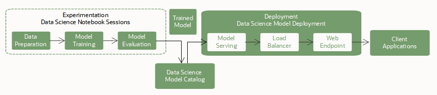
Model deployments are a managed resource in the OCI Data Science service to use to deploy machine learning models as HTTP endpoints in OCI. Deploying machine learning models as web applications (HTTP API endpoints) serving predictions in real time is the most common way that models are productionized. HTTP endpoints are flexible and can serve requests for model predictions.
Training
Training a model is the first step to deploy a model. You use notebook sessions and jobs to train open source and Oracle AutoML models.
Saving and Storing
Next, you store the trained model in the model catalog. You have these options to save a model to the model catalog:
- The ADS SDK provides an interface to specify an open source model, prepare its model artifact, and save that artifact in the model catalog.
-
You can use the OCI Console, SDKs, and CLIs to save your model artifact in the model catalog.
-
Use different frameworks such as scikit-learn, TensorFlow, or Keras.
Model deployment requires that you specify an inference conda environment in the runtime.yaml model artifact file. This inference conda environment contains all model dependencies and is installed in the model server container. You can specify either one of the Data Science conda environments or a published environment that you created.
A Model Deployment
After a model is saved to the model catalog, it becomes available for deployment as a Model Deployment resource. The service supports models running in a Python runtime environment and their dependencies can be packaged in a conda environment.
You can deploy and invoke a model using the OCI Console, the OCI SDKs, the OCI CLI, and the ADS SDK in notebook sessions.
Model deployments rely on these key components to deploy a model as an HTTP endpoint:
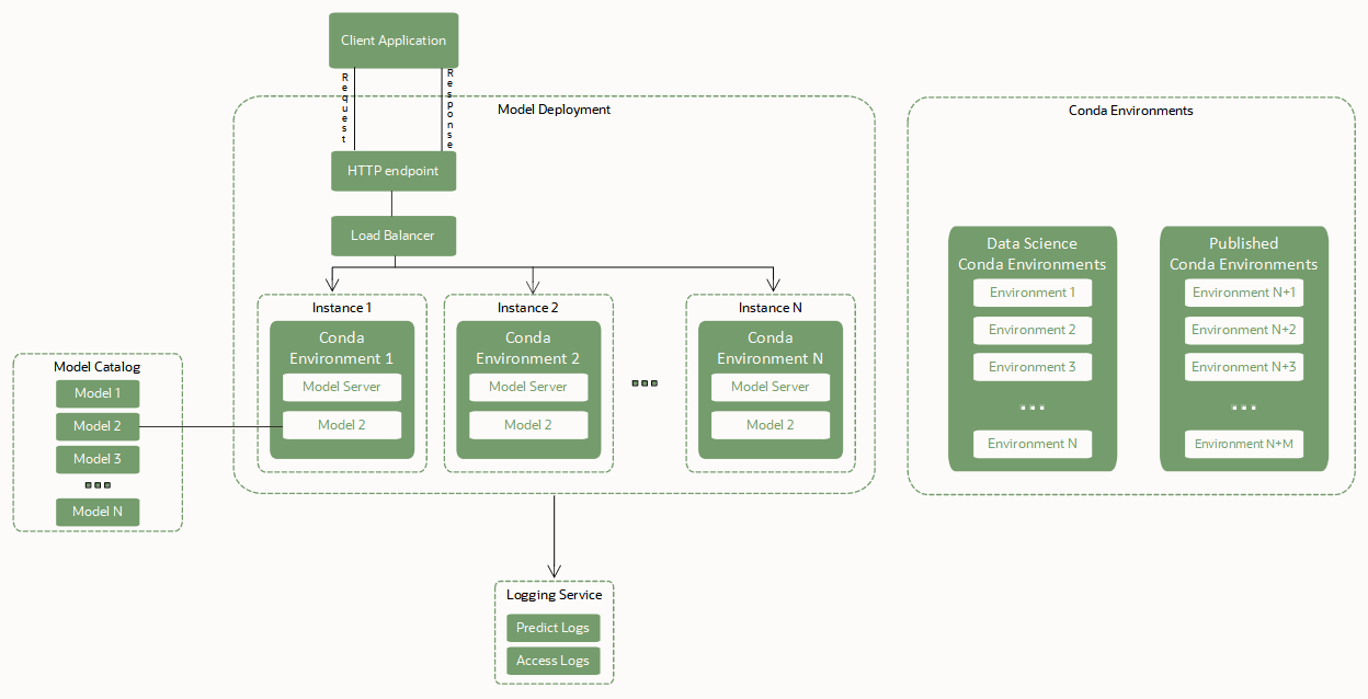
- Load Balancer.
-
When a model deployment is created, a Load Balancer must be configured. A Load Balancer provides an automated way to distribute traffic from one entry point to many model servers running in a pool of virtual machines (VMs). The bandwidth of the Load Balancer must be specified in Mbps and is a static value. You can change the Load Balancer bandwidth by editing the model deployment.
- A pool of VM instances hosting the model server, the conda environment, and the model itself.
-
A copy of the model server is made to each Compute instance in the pool of VMs.
A copy of the inference conda environment and the selected model artifact are also copied to each instance in the pool. Two copies of the model are loaded to memory for each OCPU of each VM instance in the pool. For example, if you select a VM.Standard2.4 instance to run the model server, then 4 OCPUs x 2 = 8 copies of the model are loaded to memory. Several copies of the model help to handle concurrent requests that are made to the model endpoint by distributing those requests among the model replicas in the VM memory. Ensure that select a VM shape with a large enough memory footprint to account for those model replicas in memory. For most machine learning models with sizes in MBs or the low GBs, memory is likely not an issue.
The Load Balancer distributes requests made to the model endpoint among the instances in the pool. We recommend that you use smaller VM shapes to host the model with a larger number of instances instead of selecting fewer though larger VMs.
- Model artifacts in the model catalog.
-
Model deployment requires a model artifact that's stored in the model catalog and that the model is in an active state. Model deployment exposes the
predict()function defined in the score.py file of the model artifact. - Conda environment with model runtime dependencies.
-
A conda environment encapsulates all the third-party Python dependencies (such as Numpy, Dask, or XGBoost) that a model requires. The Python conda environments support Python versions
3.7,3.8,3.9,3.10, and3.11. The Python version you specify withINFERENCE_PYTHON_VERSIONmust match the version used when creating the conda pack.Model deployment pulls a copy of the inference conda environment defined in the runtime.yaml file of the model artifact to deploy the model and its dependencies. The relevant information about the model deployment environment is under the
MODEL_DEPLOYMENTparameter in theruntime.yamlfile. TheMODEL_DEPLOYMENTparameters are automatically captured when a model is saved using ADS in a notebook session. To save a model to the catalog and deploy it using the OCI SDK, CLI, or the Console, you must provide aruntime.yamlfile as part of a model artifact that includes those parameters.Note
For all model artifacts saved in the model catalog without a
runtime.yamlfile, or when theMODEL_DEPLOYMENTparameter is missing from theruntime.yamlfile, then a default conda environment is installed in the model server and used to load a model. The default conda environment that's used is the General Machine Learning with Python version 3.8.Use these conda environments:
- Data Science conda environments
-
A list of the conda environments is in Viewing the Conda Environments.
In the following example, the
runtime.yamlfile instructs the model deployment to pull the published conda environment from the Object Storage path defined byINFERENCE_ENV_PATHin ONNX 1.10 for CPU on Python 3.7 .MODEL_ARTIFACT_VERSION: '3.0' MODEL_DEPLOYMENT: INFERENCE_CONDA_ENV: INFERENCE_ENV_SLUG: envslug INFERENCE_ENV_TYPE: data_science INFERENCE_ENV_PATH: oci://service-conda-packs@id19sfcrra6z/service_pack/cpu/ONNX 1.10 for CPU on Python 3.7/1.0/onnx110_p37_cpu_v1 INFERENCE_PYTHON_VERSION: '3.7' - Your published conda environments
-
You can create and publish conda environments for use in model deployments.
In the following example, the
runtime.yamlfile instructs the model deployment to pull the published conda environment from the Object Storage path defined byINFERENCE_ENV_PATH. It then installs it on all instances of the pool hosting the model server and the model itself.MODEL_ARTIFACT_VERSION: '3.0' MODEL_DEPLOYMENT: INFERENCE_CONDA_ENV: INFERENCE_ENV_SLUG: envslug INFERENCE_ENV_TYPE: published INFERENCE_ENV_PATH: oci://<bucket-name>@I/<prefix>/<env> INFERENCE_PYTHON_VERSION: '3.7'
For all model artifacts saved in the catalog without a
runtime.yamlfile, model deployments also use the default conda environment for model deployment. A model deployment can also pull a Data Science conda environment or a conda environment that you create or change then publish. - Zero Downtime Operations
-
Zero downtime operations for model deployments mean that the model inference endpoint (predict) can continuously serve requests without interruption or instability.
Model deployments support a series of operations that can be done while maintaining no downtime. This feature is critical for any application that consumes the model endpoint. You can apply zero downtime operations when the model is in an active state serving requests. Use these zero downtime operations to swap the model for another one, change the VM shape, and the logging configuration while preventing downtime.
- Logging Integration to Capture Logs Emitted from Model Deployment
-
You can integrate model deployments with the Logging service. Use this optional integration to emit logs from a model and then inspect these logs.
- Custom container with model runtime dependencies
-
A custom container encapsulates all the necessary third-party dependencies that a model requires for inference. It also includes a preferred inference server, such as Triton inference server, TensorFlow serving, ONNX runtime serving, and so on.
- GPU Inference
-
Graphical Processing Unit inference is widely used for compute intensive models such as LLaMa or Generative Pre-trained Transformers.
- Custom Egress
- You can select between service-managed networking or customer-managed networking, similar to custom egress with Jobs and Notebooks.
- Private Endpoint
-
To enhance security and control, you can access model deployments through a private network (private model deployment). With support for private endpoints, your inference traffic stays securely within the private network. For more information, see the section Creating a Private Endpoint and Creating a Model Deployment to configure a model deployment with a private endpoint.
Model Deployments Details
After you select a project, the Project details page is displayed with a list of notebook sessions and other resources such as model deployments.
Select Model deployments to go to the model deployments details page for the selected compartment, where you can:
-
Create model deployments.
-
Select a model deployment to view its details and work with it.
-
Use the to view details, edit, move a model deployment, or delete a model deployment.
-
OCID: The OCID of a resource. A shortened version of the OCID is displayed though you can use Show and Hide to switch the display of the OCID. Use the Copy link to save the entire OCID to the clipboard to paste it elsewhere. For example, you could paste into a file and save it, then use it in model scripts.
-
Use the List Scope filter to view model deployments associated with the selected project in another compartment.
-
Filter model deployments by status using the State list. The default is to view all status types.
-
When tags applied to model deployments, you can further filter model deployments by clicking add or clear next to Tag Filters.
-
Select other Data Science resources, such as models, model deployments, and notebook sessions.